GPU benchmarking and how to choose a GPU framework

This is the final installment of our 4-part series on GPU programming. Catch up on the previous articles:

• What is GPU programming

• Your first GPU algorithm: Scan/prefix sum

• Your second GPU algorithm: Quicksort

With those topics covered, we can now move on to the subject of this article: how to choose a GPU framework/library.

How to choose a GPU framework

Generally, when you’re benchmarking some GPU code, you want to make sure to do the following:

• Run the algorithm more than once, and get the median/quartiles, or mean/stdev of each of the running times.
• Synchronize your CUDA kernels, to make sure the program has fully finished executing—by default CUDA will launch kernels asynchronously (in the background) so that the host can continue processing things.
• Clear the L2 cache, usually by running a bogus script that requires enough cache memory to clear everything.
• Warm up each of your scripts—this is especially important for Triton, because the autotuner needs to conduct a full grid search every time to determine the right hyperparameters for each run (e.g., BLOCK_SIZE, etc.). Luckily, if you're using Triton and choose to compile ahead of time, this will be done on compilation time instead. 
• Ensure you have enough disk space—strangely, this ended up being a big deal for us on our NVIDIA machine, where Triton was severely underperforming (factor of 50x) until we cleared up enough disk space. We speculate that perhaps the Triton JIT needed disk space in order to run effectively, whereas the Torch JIT didn’t. However, we’re not entirely sure. 
• Use torch.cuda.Event(enable_timing=True) to do timings, because this might be slightly more accurate than using time.time(), for example.

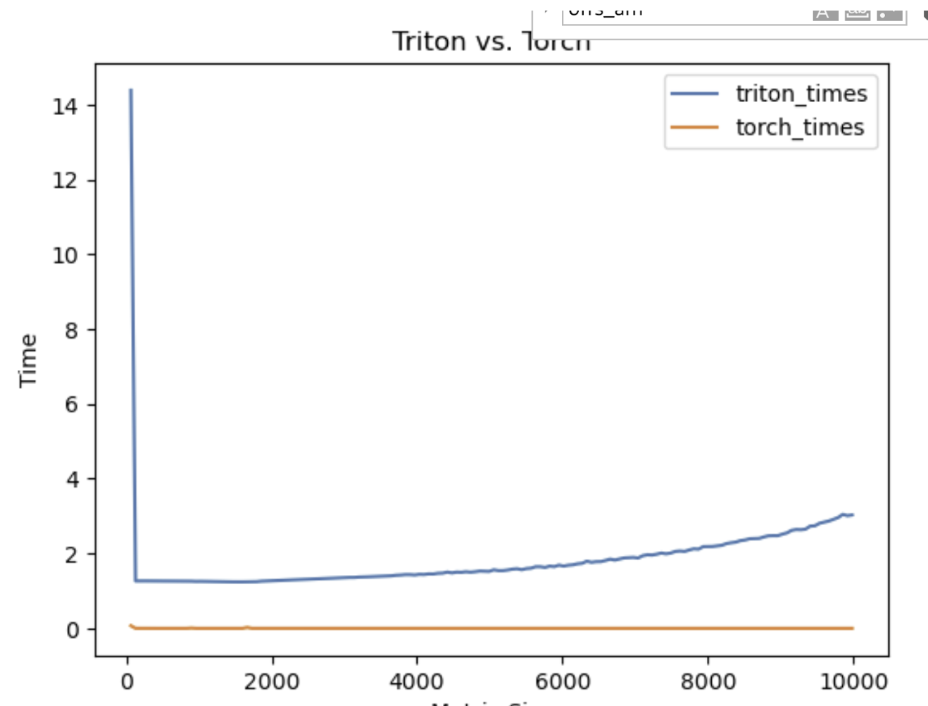
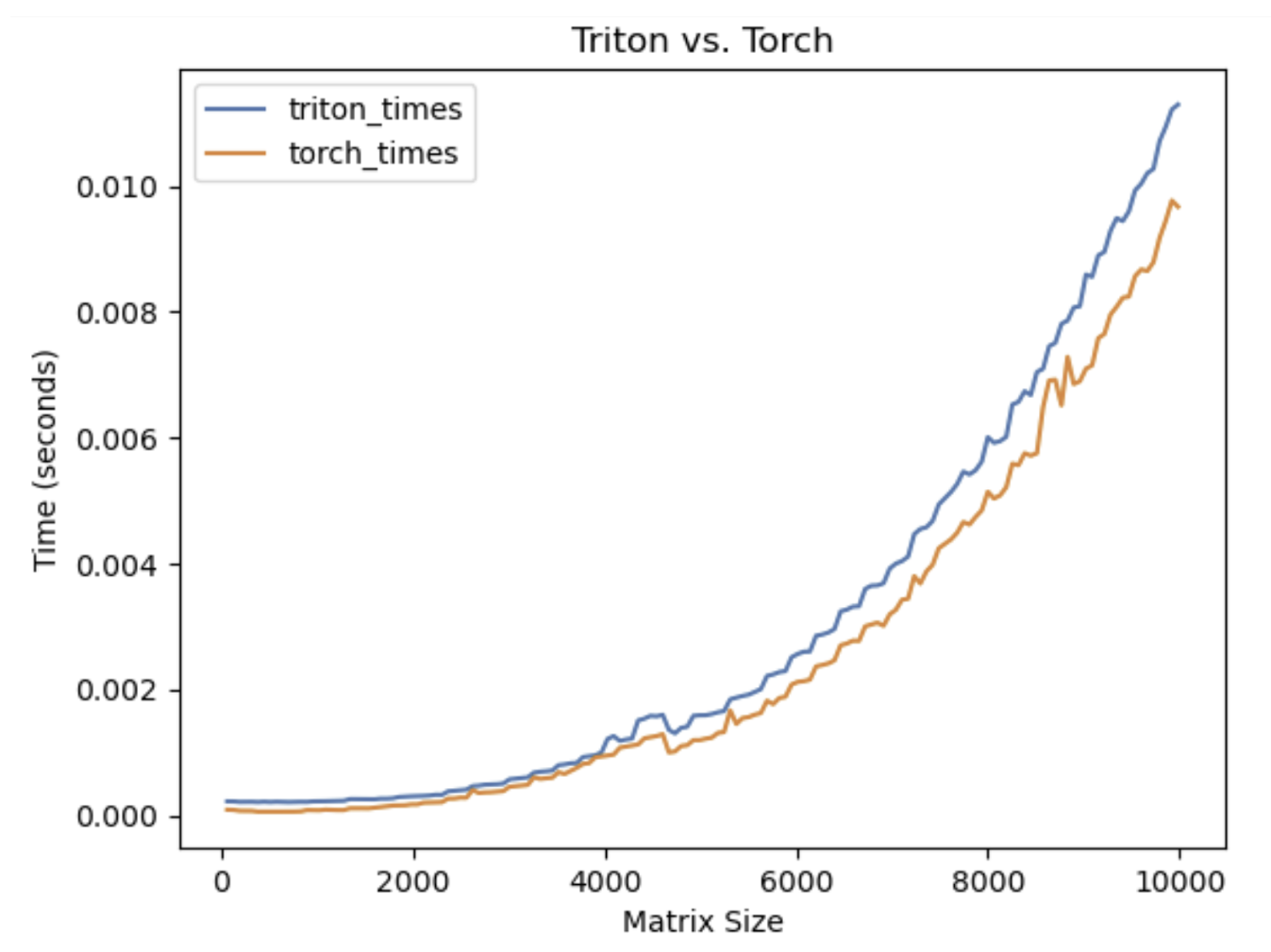
You can see an example of the results a bad benchmark produces in Figure 1, and an example of a good benchmark in Figure 2. 

Created by Kenneth Ge,

Created by Kenneth Ge,

Implementation details

We can clear the cache by forcing a new array into memory, as follows:

cache_size = 256 * 1024 * 1024
cache = torch.empty(int(cache_size), dtype=torch.int8, device='cuda')
cache.zero_()

We can queue synchronized CUDA timing events as follows:

start_event = torch.cuda.Event(enable_timing=True)
start_event.record()
start_event.elapsed_time(end_event)

When we call event.record(), we essentially queue up a record event in CUDA, so that instead of needing to wait for the kernel to synchronize, as soon as the previous queued operation has completed, the CUDA driver will record the current time. 

Differences between frameworks

There are a handful of differences between each framework, detailed below.

Triton

Triton claims to be more efficient because instead of specifying individual instructions, you specify block instructions. Thus, it will automatically parallelize within each block for you, and you won’t have to worry about any data race conditions, and etc. 

The downside is that to get the most of it, you really must use block operations. So, you must: 

•  Be familiar with numpy/torch block ops, and how to work with numpy-style indexing.
• Have a data workload that can be defined using only the pre-defined torch block operations.

In certain implementations, Triton can use block operations to optimize low-precision floating point operations. For example, if you’re using 8-bit or 4-bit floats, it’s very possible that Triton block operations will automatically optimize this for you by e.g. going 64 bits at a time, rather than losing efficiency by running one thread per 4-bit item. 

However, one really important practical consideration is that, in many of these workloads, if you’re being limited to just PyTorch/Triton block functions, it is often easier to just use torch.compile to build the kernel automatically, or even skip the kernel altogether and just use a series of torch.XX operations instead. Also, if you end up doing any custom functions (such as Conway’s Game of Life), you may not be able to take full advantage of the automatically parallelized bock operations. 

Also, race conditions can still occur if they happen across blocks. For example, when I was developing a matrix multiplication algorithm, I came across a race condition with the following code:

@triton.jit
def matrix_mult(A, B, C, M, K, N, BLOCK_SIZE_M : tl.constexpr, BLOCK_SIZE_K : tl.constexpr, BLOCK_SIZE_N : tl.constexpr):
    """
    C := A x B
    """
    pid_m = tl.program_id(axis=0)
    pid_k = tl.program_id(axis=1)
    pid_n = tl.program_id(axis=2)

    # current block m-wise
    offs_am = (pid_m * BLOCK_SIZE_M + tl.arange(0, BLOCK_SIZE_M)) % M
    # current block n-wise
    offs_bn = (pid_n * BLOCK_SIZE_N + tl.arange(0, BLOCK_SIZE_N)) % N
    # current block k-wise
    offs_k = (pid_k * BLOCK_SIZE_K + tl.arange(0, BLOCK_SIZE_K)) % K

    # get m x k block in A
    a_ptrs = A + (offs_am[:, None] * K + offs_k[None, :] * 1)
    # get k x n block in B
    b_ptrs = B + (offs_k[:, None] * N + offs_bn[None, :] * 1)
    
    # Load the next block of A and B, generate a mask by checking the K dimension.
    # If it is out of bounds, set it to 0.
    a = tl.load(a_ptrs, mask=offs_k[None, :] < K, other=0.0)
    b = tl.load(b_ptrs, mask=offs_k[:, None] < K, other=0.0)

    c_start = C + BLOCK_SIZE_M * pid_m * N + pid_n * BLOCK_SIZE_N * 1

    this_block = c_start + tl.arange(0, BLOCK_SIZE_M)[:, None] * N + tl.arange(0, BLOCK_SIZE_N)[None, :] * 1

    # We accumulate along the K dimension.
    ans = tl.dot(a, b)
    tl.store(this_block, tl.load(this_block) + ans)

This is because multiple blocks were accessing the same block indices in our output array C, and attempting to each read, add, and write to this block. The best way to avoid this is unfortunately to redesign your code. A more thorough review of Triton matrix multiplication and performance optimizations without race conditions can be found here. 

OpenCL

Unlike Triton, OpenCL is a lot more low-level. Even in PyOpenCL, you end up writing GLSL shader code for kernels, and you also need to worry about setting up a context etc. On the other hand, with Triton, you simply use PyTorch as normal, and simply make sure to move your memory over to the device (i.e., device=’cuda’). 

However, OpenCL can actually feel easier to code for certain tasks, because you write kernels that execute for every thread, rather than for every block like in Triton. This makes it easier for reason about what you’re doing in situations like this.

Triton:

@triton.jit
def scan(Y, nextY, stride, BLOCK_SIZE: tl.constexpr):
    pid_row = tl.program_id(0)

    for j in tl.static_range(BLOCK_SIZE):
        current_idx = pid_row * BLOCK_SIZE + j
        if current_idx - stride >= 0:
            Yj = tl.load(Y + current_idx)
            Yjminstride = tl.load(Y + current_idx - stride)
            
            tl.store(nextY + current_idx, Yj + Yjminstride)
        else:
            tl.store(nextY + current_idx, tl.load(Y + current_idx))

OpenCL:

__kernel void psum_step(__global float *src, __global float *dest, int stride)
{
    int gid = get_global_id(0);

    if(gid - stride >= 0)
        dest[gid] = src[gid] + src[gid - stride];
}

The above is a kernel representing one step in a prefix sum. Notice that in Triton you have to worry about the block operation, whereas in OpenCL you can assume that you’re working directly on each individual index. Both approaches will have their pluses and minuses for different types of problems. Also notice that OpenCL allows for much more convenient syntax, whereas in Triton you must use fairly convoluted operations like tl.store, tl.load, tl.static_range, and etc. 

Notice that it’s not clear whether the Triton version is necessarily even more efficient—because it works on a per-block basis, it is entirely possible that the entire function is just running on a single thread, which has to process the entire block size. The Triton team claims that they have done some serious work under the hood in terms of automatic parallelism and compiler optimizations, but due to a lack of documentation, it is difficult to determine which custom block operations will be fully parallelized. 

However, one of the disadvantages of working at such a low level is needing to worry about corrupted data if your types don’t match. Take a look at the following code:

import numpy as np
import pyopencl as cl

ctx = cl.create_some_context()
queue = cl.CommandQueue(ctx)

mf = cl.mem_flags

prg = cl.Program(ctx, """__kernel void fill(__global float *res_g)
{
    int gid = get_global_id(0);

    res_g[gid] = 1.0;
}""").build()

# create numpy starting array
a_np = np.arange(8)
a_g = cl.Buffer(ctx, mf.READ_WRITE | mf.COPY_HOST_PTR, hostbuf=a_np)
res_g = cl.Buffer(ctx, mf.READ_WRITE, a_np.nbytes)
res_np = np.empty_like(a_np)

prg.fill(queue, res_np.shape, None, res_g)

cl.enqueue_copy(queue, res_np, res_g)

print(res_np)
print(a_np)

This benign-looking program simply creates a numpy array using the arange function, then creates another buffer the same size, called res_np, and attempts to use the fill kernel to fill all elements in res_g to 1.0. The output is as follows:

[4575657222473777152 4575657222473777152 4575657222473777152
 4575657222473777152                   0                   0
                   0                   0]
[0 1 2 3 4 5 6 7]

The kernel didn’t work! In fact, the data in the resulting buffer is completely garbled. It turns out, the reason this didn’t work is because our kernel expects to take in 32-bit floats, but np.arange uses int64 by default. If we simply add the line a_np = a_np.astype(np.float32), we will get the correct answer. This bug is entirely non-obvious. In fact, I spent about two days getting stuck here. 

Numba

Surprisingly, Numba is actually one of the most highly recommended and well-documented tools that Nvidia mentions in its Python GPU programming page. 

It combines the low-level control of CUDA or OpenCL, with the ease of Python. It functions similar to Triton in that you define a function with a custom annotation, and don’t have to deal with an environment other than moving data to/from the GPU. 

Overall, in a practical setting, I would recommend using Numba for a few reasons:

• Numba is incredibly well-supported, on both the GPU and the CPU side. So this library is going to likely be less buggy, and more likely to work.
• Because it transpiles down to CUDA/HCC code under the hood, it’s more likely to benefit from optimizations, that are otherwise unavailable to OpenCL due to its age and neglect.
• It still gives you that same level of control that CUDA/OpenCL does, without forcing you to use the block operations that Triton does. Not that block operations are bad—but the optimizations come at the cost of potentially more difficult development.

Here’s a Numba kernel for the prefix sum:

@cuda.jit
def numba_psum(input_array, output_array, stride, N):
    # Thread id in a 1D block
    tx = cuda.threadIdx.x
    # Block id in a 1D grid
    ty = cuda.blockIdx.x
    # Block width, i.e. number of threads per block
    bw = cuda.blockDim.x
    # Compute flattened index inside the array
    pos = tx + ty * bw

    back_pos = pos - stride

    if pos >= N:
        return
    
    if back_pos < 0:
        output_array[pos] = input_array[pos]
    else:
        output_array[pos] = input_array[pos] + input_array[back_pos]

Conclusion

Congrats! You've completed this four-part GPU getting started guide. Now, you have a good grasp on some of the foundational algorithms and techniques used in parallel programming. With these tools, I hope you will be one step closer toward writing the next generation of high-performance algorithms.