Your second GPU algorithm: Quicksort

Using the algorithm for prefix sum/scan, covered in the previous module, we’re going to now write an algorithm for quicksort.

This is part 3 of a 4-part series. Catch up on the previous articles:

• What is GPU programming

• Your first GPU algorithm: Scan/prefix sum

The quicksort algorithm

The reason we’re doing quicksort, rather than something like merge sort, is that it’s very easy to parallelize– once you partition the array, each partition can be sorted completely independently. Plus, it is efficient in the average case, especially if you use randomness to select your pivot. 

Recall that the pseudocode for quicksort is as follows:

def quicksort(array, BLOCK_SIZE):
	p = randomly select pivot from array
	let below_arr = global, reused array that stores the number of items in each block less than p
 	let above_arr = global, reused array that stores the number of items in each block above p
	# parallelized using GPU kernel
	for each block:
		count number of items < p, save to below_arr
		count number of items > p, save to above_arr
	
	# parallelized using GPU kernel
	let offset_below = prefix_sum(below_arr)
	let offset_above = prefix_sum(above_arr)

	# parallelized using GPU kernel
	for each block b:
		idx_below = offset_below[b]
		idx_above = num_items_below_p + offset_above[b]
		for each item i in block:
			if i < p:
				array[idx_below++] = i
			else:
				array[idx_above++] = i

Here, I've added annotations as well, for areas that we're able to accelerate using the GPU. Essentially, this algorithm is equivalent to the CPU version of quicksort, but we use the GPU to speed up the partitioning step. Then, we can call quicksort again on both sub-partitions simultaneously, and run them in parallel. 

The goal with GPU partitioning is that we want to be able to have each block work independently of the next. So, each block will simply place all of its contained elements into the correct position in the array. However, this becomes tricky because we don’t necessarily know what those positions are. 

So, we will first count the number of elements above and below the partition element in each block. Then, we use our prefix sum to determine the total number of elements that are above or below our pivot, in all the blocks prior to each block. This becomes our offset, which we use to determine where to place all of our elements. 

Example

Let's take a look at an example. Say we have the pivot p = 3, the array arr = [6, 5, 4, 2, 1, 0], and a total of 3 blocks. Let's let each block be two consecutive elements. 

We first count the number of elements in each block that are above and below the pivot. So, we have below_arr = [0, 1, 2], and above_arr = [2, 1, 0]. 

Then, we count the total number of elements that are below the pivot, which is equal to sum(below_arr) = 3. 

Using this information, we then calculate the offsets that each new block will occupy-- one offset for where elements below the array will be, and one offset for where elements above the array will be. Notice that this is equivalent to the prefix sum, except this time we don't include the current element: offset_below = [0, 0, 1], and offset_above = 3 + [0, 2, 3] = [3, 5, 6]. 

Now, our GPU kernels can execute each block independently, and use these offsets to place elements into the right place in our final sorted array. This final process is very similar to what you might do on the CPU. 

Below are some Triton kernels for doing the above partitioning step.

Prefix sum:

@triton.jit
def scan(Y, nextY, stride, BLOCK_SIZE: tl.constexpr):
    pid_row = tl.program_id(0)

    for j in tl.static_range(BLOCK_SIZE):
        current_idx = pid_row * BLOCK_SIZE + j
        if current_idx - stride >= 0:
            Yj = tl.load(Y + current_idx)
            Yjminstride = tl.load(Y + current_idx - stride)
            
            tl.store(nextY + current_idx, Yj + Yjminstride)
        else:
            tl.store(nextY + current_idx, tl.load(Y + current_idx))

def triton_pref_sum(X):
    Y = torch.clone(X)
    Ynext = torch.empty_like(Y, device='cuda')
    n = X.shape[0]
    stride = 1
    for i in range(0, int(math.log2(n))):
        scan[(math.ceil(n / BLOCK_SIZE),)](Y, Ynext, stride, BLOCK_SIZE)
        stride *= 2
        Ynext, Y = Y, Ynext

    return Y

Count above/below:

@triton.jit
def count(offset, X, under_pivot, over_pivot, pivot_idx, N, BLOCK_SIZE: tl.constexpr):
    pid = tl.program_id(0)
    block = offset + pid * BLOCK_SIZE + tl.arange(0, BLOCK_SIZE)

    item = tl.load(X + block, mask=block<offset + N, other=float('nan'))
    num = tl.sum(tl.where(item < tl.load(X + offset + pivot_idx), 1, 0))

    tl.store(under_pivot + pid, num)
    tl.store(over_pivot + pid, tl.sum(tl.where(block<offset+N, 1, 0)) - num)

Partition:

@triton.jit
def triton_partition(offset, X, Y, pivot_idx, count_under_pivot, count_over_pivot, start_indices, start_indices2, total_before, N, BLOCK_SIZE: tl.constexpr):
    pid = tl.program_id(0)
    
    startidx = tl.load(start_indices + pid).to(tl.int64) - tl.load(count_under_pivot + pid).to(tl.int64)
    startidx2 = tl.load(total_before).to(tl.int64) + tl.load(start_indices2 + pid).to(tl.int64) - tl.load(count_over_pivot + pid).to(tl.int64)

    pivot = tl.load(X + offset + pivot_idx)
    
    for i in tl.static_range(BLOCK_SIZE):
        pos = pid * BLOCK_SIZE + i
        if pos < N:
            value = tl.load(X + offset + pos)
            if value < pivot:
                tl.store(Y + offset + startidx, value)
                startidx += 1
            else:
                tl.store(Y + offset + startidx2, value)
                startidx2 += 1

def partition(X, Y, left, right):
    """
    left and right are inclusive
    """
    
    N = right - left + 1
    pivot_idx = np.random.randint(N)
    pivot = X[left + pivot_idx]

    count_under_pivot = torch.zeros((math.ceil(N / BLOCK_SIZE)), device='cuda')
    count_over_pivot = torch.zeros((math.ceil(N / BLOCK_SIZE)), device='cuda')

    count[(math.ceil(N / BLOCK_SIZE),)](left, X, count_under_pivot, count_over_pivot, pivot_idx, N, BLOCK_SIZE)

    count_under_pivot = count_under_pivot.long()
    count_over_pivot = count_over_pivot.long()

    start_indices = triton_pref_sum(count_under_pivot)
    start_indices2 = triton_pref_sum(count_over_pivot)

    total_before = start_indices[-1]

    triton_partition[(math.ceil(N / BLOCK_SIZE),)]\
    (left, X, Y, pivot_idx, count_under_pivot, count_over_pivot, \
     start_indices, start_indices2, total_before, N, BLOCK_SIZE)

    return pivot, total_before.item()

Reduce/fold

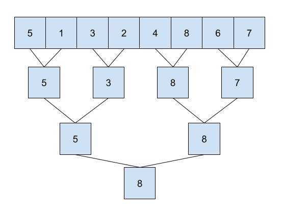
In general, we can think of GPU computation as a tree. Each level represents some computation you want to do. For example, in quicksort, each level represents one partition step. 

Each time you call a GPU kernel, you can think of it as doing one entire level of the tree at once. That way, you can speed up the algorithm by simply doing O(log n) GPU computations. 

We’re going to use this technique to write a parallel reduce algorithm. Recall that the reduce function simply takes an array, and reduces it down to a singular value, based on some series of computations. For example, one possible reduction would be taking the sum, and another would be taking the max. In general, the options are quite limitless, since you can do whatever computation you want. 

Here, we write a parallel algorithm for the reduce function, that works on associative operators. We do this by treating the array as the leaf nodes of our tree, and collapsing it down layer by layer into a single node. 

For example, in Figure 1, we can see what the overall structure of what a maxfold might look like.

Created by Kenneth Ge,

Implementation of such an algorithm is left up to you; it involves the same swapping procedure we did for the scan kernel. 

Game of Life

For this module, we leave the Game of Life algorithm as an exercise to the reader! A hint is that you should try to figure out how to represent a 2D index as a single one-dimensional number. 

To learn more about using GPUs, try this hands-on learning path: Configure a Jupyter notebook to use GPUs for AI/ML modeling