Page
Clone a GitHub repository into your environment
Your Developer Sandbox environment is complete. Now it's time to populate it.
In order to get full benefit from taking this lesson, you need to:
- Have an OpenShift cluster from the Developer Sandbox
In this lesson, you will:
- Learn how to clone a GitHub repository
- Learn how to submit repairs
- Learn how to expose the model as an API
Clone a GitHub repository into your environment
It’s pretty empty right now, so the first thing you need to do is bring the content of the workshop inside this environment.
On the left toolbar, select the GitHub icon (Figure 5).

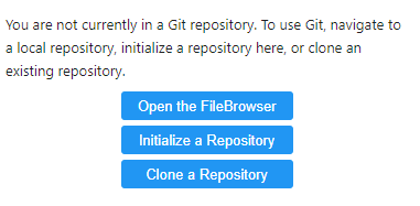
Figure 5: Select the GitHub icon on the lab toolbar. Select Clone a Repository (Figure 6).

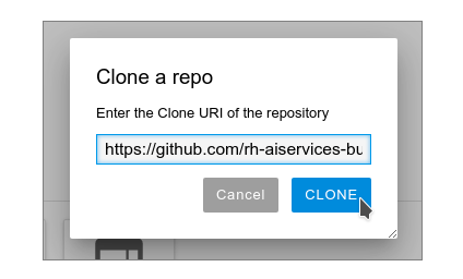
Figure 6: Select "Clone a Repository" at the bottom of the screen for the current image. Enter the URL https://github.com/rh-aiservices-bu/metrobus-repairs-nlp-workshop.git and select CLONE. (Figure 7).

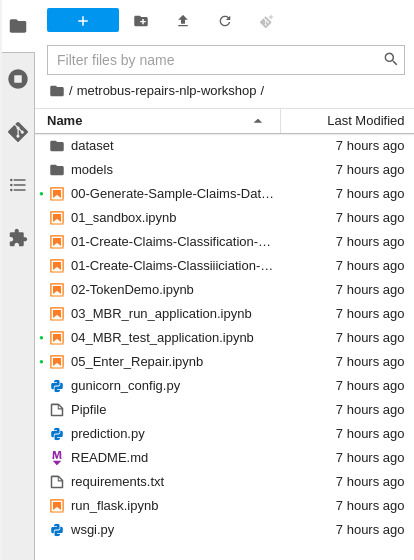
Figure 7: Enter the URL and click CLONE. Cloning the repository takes a few seconds, after which you can double-click and navigate (Figures 8 and 9) to the newly-created folder,
metrobus-repairs-nlp-workshop.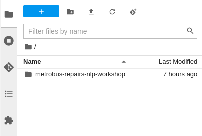
Figure 8: Double-click the repository you've cloned. 
Figure 9: Navigate to the newly-created folder.


What’s a notebook?
A notebook is an environment with cells that can display formatted text or code (Figure 10).
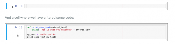
Code cells contain code that can be run interactively. That means you can modify the code, then run it. The code will not run on your computer or in the browser, but directly in the environment to which you are connected; OpenShift AI in our case.
To run a code cell, just click in it or on the left side of it, and then click the Run button from the toolbar. You can also press Ctrl+Enter to run a cell, or Shift+Enter to run the cell and automatically select the following one.
The Run button on the toolbar looks as shown in Figure 11.
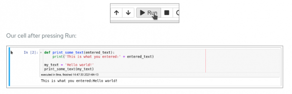
Running the cell ends by showing the result of the code that was run in that cell, as well as information about when this particular cell has been run. You can also enter notes into a cell by switching the cell type in the menu from Code to Markup.
Info alert: Note: When you save a notebook, both the code and the results are saved. So you can reopen the notebook to look at the results without having to run the program again, and while still having access to the code.
Time to play
Now that we have covered the basics, give notebooks a try. In your Jupyter environment (the file explorer-like interface), there is a file called 01_sanbdbox.ipynb. Double-click on it to launch the notebook, which will open another tab in the content section of the environment.
Feel free to experiment, run the cells, add some more cells, and create functions. You can do whatever you want, because the notebook is your personal environment, and there is no risk of breaking anything or affecting other users. This environment isolation is a great advantage of OpenShift AI.
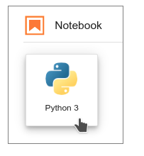
You can create a new notebook by selecting File→New→Notebook from the menu on the top left, then selecting a Python 3 kernel. This selection asks Jupyter to create a new notebook that runs the code cells using Python 3. You can also create a notebook by simply clicking on the icon in the launcher. (Figure 12)
To learn more about notebooks, head to the Jupyter site. Now that you’re more familiar with notebooks, you’re ready to go to the next section.
Submitting metro bus repairs using NLP
Now that you know how the environment works, the real work can begin.
Still in your environment, open the
01-Create-Claims-Classification.ipynbfile, and follow the instructions directly in the notebook. After you run the code in the notebook, it will look like Figure 13.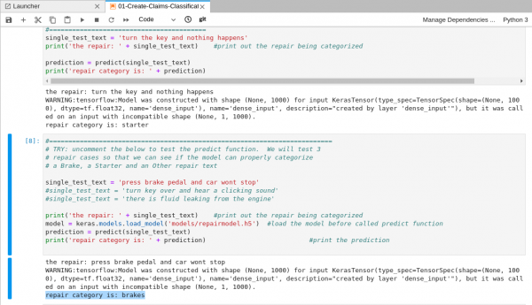
Figure 13: The results after you run the code in the notebook. Once you are finished, you can come back here and head to the next section.

Expose the model as an API
In the previous section, we learned how to create the code that classifies a repair based on the free text we enter. But we can't use a notebook directly like this in a production environment. That means we will learn how to package this code as an API that you can directly query it from other applications.
Some quick notes
- The code that we wrote in the notebook has been repackaged as a single Python file,
prediction.py. Basically, the file combines the code in all the cells of the notebook. - To use this code as a function you can call, we added a function called predict that takes a string as an input, classifies the repair, and sends back the resulting classification.
- Open the file directly in JupyterLab, and you should recognize our previous code along with this new additional function.
- There are other files in the folder that provide functions to launch a web server, and we will use those files to serve our API.
The steps
- Open the
03_MBR_run_application.ipynbfile and follow the instructions directly in the notebook. - Our API will be served directly from our container using Flask, a popular Python web server. The Flask application, which will call our prediction function, is defined in the
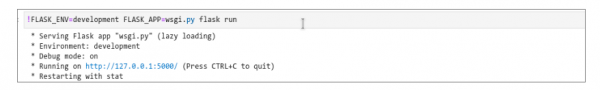
wsgi.pyfile. - When you execute the following cell, it will be in a permanent running state. That's normal, because the web server process will keep running. When you are finished with the test, you can simply select the cell and click the Stop button (next to Run).
Launch the Flask application (Figure 14).

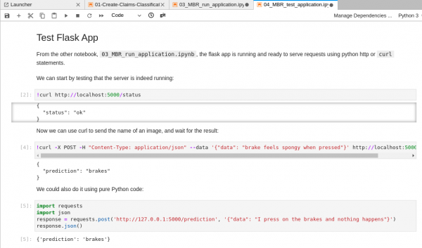
Figure 14: Launch the Flask application when you are ready to open the file. Then query the API (Figure 15).

Figure 15: Query the API after launching the server. Once you are finished, you can come back here and head to the next step.
- You are ready to test the Flask application. Open the Jupyter notebook named
04_MBR_test_application.ipynband follow the instructions in the notebook.
Congratulations. You have set up your sandbox environment and populated it. Your next step is to build the application in Red Hat OpenShift.
