Prerequisites and step-by-step guide

Prerequisites:

• Fundamentals of OpenShift AI learning exercise
• Red Hat Developer Sandbox
• Red Hat OpenShift cluster
• GitHub
• Prior knowledge of Python

Launch JupyterLab to build an image prediction model

1. Launch an Jupyter notebook with TensorFlow server image

This learning exercise delves into image prediction within the OpenShift AI platform. We'll explore how to train a model using a dataset of cat and dog images to achieve this task. To get started, we'll establish a new Data Science project within OpenShift AI that leverages a pre-configured TensorFlow image. This image provides a ready-to-use environment for building and training your machine learning models.

Creating a New Workbench in OpenShift AI

• Log in and navigate to the OpenShift AI platform to access the OpenShift AI Dashboard.
• Locate the "Data Science Projects" option in the left-hand menu and click on it.

Choose a Project:

• Click on the pre-created Data Science project associated with your username.

Create a Workbench:

• Within the chosen project, navigate to the "Workbenches" tab.
• Click on "Create Workbench" to initiate the workbench creation process.

Configure the Workbench:

• Provide a descriptive name for your workbench.
• Under "Notebook image," select "TensorFlow" and keep the version set to "Recommended".
• In the "Deployment size" section, choose "Medium" for the container size.
• Change the "Cluster storage" setting to 10Gi.

Finalize Creation: 

• Click on "Create Workbench" to initiate the creation process and launch your new workbench environment, as shown in Figure 1 below.

Verify Workbench Status:

• Once you click "Create Workbench", monitor the workbench status. It should eventually transition to "Running", indicating successful creation.

Access Jupyter Notebook:

• Locate the "Open" button displayed next to your newly created workbench (refer to the provided image for reference). Click on this button.
• You might encounter a permission prompt. Select the option "Allow selected permissions" to grant the necessary access.

Your Jupyter Notebook environment will come pre-configured with TensorFlow and its dependencies (Figure 2).

The Jupyter notebook offers the ability to fetch or clone existing GitHub repositories, just like any standard IDE. Follow these instructions to clone an existing simple ML/AI project into the notebook.

• At the top, click on the "Git Clone" icon.
• In the popup window, enter the following GitHub URL: https://github.com/redhat-developer-demos/openshift-ai.git
• Click the "Clone" button as shown below.
• Navigate to the "openshift-ai/2_Cat-dog-prediction" directory.

2. Access to datasets

We are collecting the dataset of images from Kaggle. Kaggle is the world's largest data science community tool. To get access to Kaggle, use this link. 

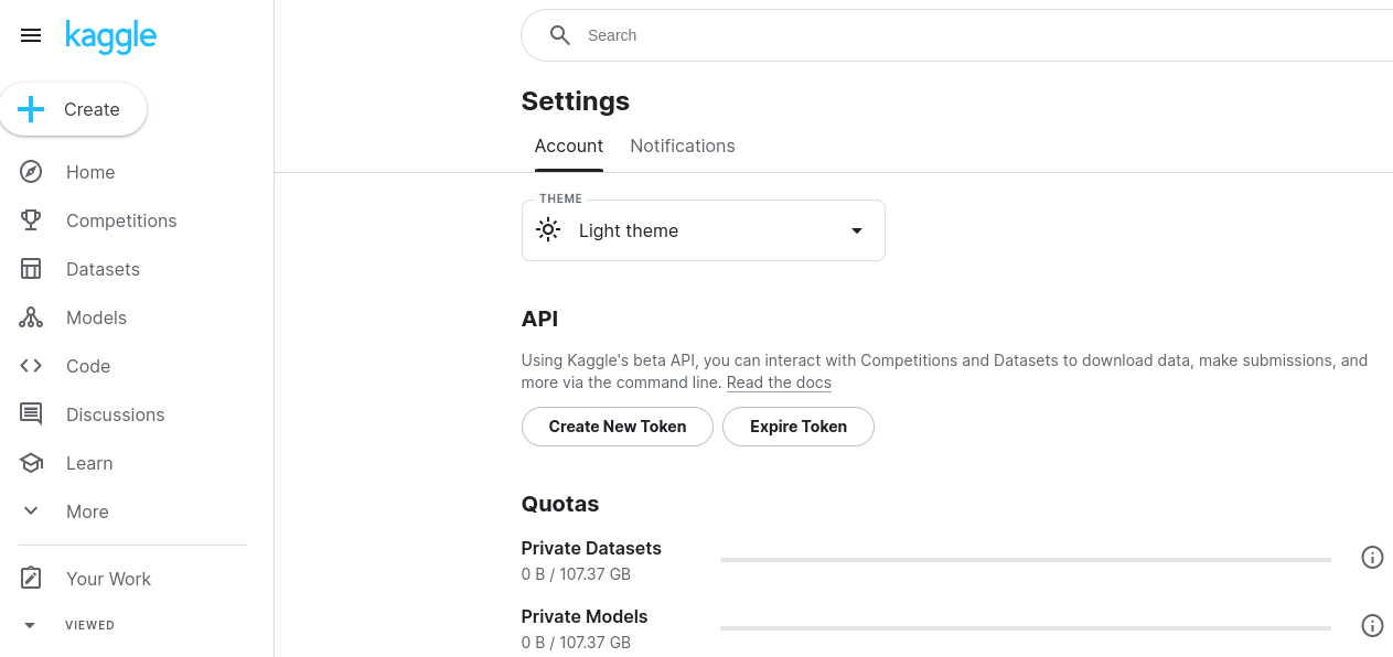
Obtaining Your Kaggle API Token

To interact with the Kaggle API from your Jupyter Notebook environment, you'll need a personal API token. Here's how to obtain it:

• Access Your Kaggle Account Settings: Navigate to your Kaggle account settings. You can typically access these settings by clicking on your profile icon in the top right corner and selecting "Account" or a similar option.
• Generate Your Token: Within the API section, find a button labeled "Create New Token". Clicking this button will initiate the token creation process.
• Download the kaggle.json File: Upon creating the token, your web browser should automatically download a file named "kaggle.json". This file contains your unique API credentials and is essential for authorizing your Jupyter Notebook to access Kaggle datasets.

3. Image prediction python code

This section delves into image prediction using TensorFlow and leverages a dataset from the Kaggle platform. We'll train a model to classify cat and dog images, assigning "0" to cat images and "1" to dog images. This serves as a foundational example of supervised machine learning and showcases the capabilities of OpenShift AI.

Select the "Notebook Python 3.9" option from the landing page of Jupyter Notebook.

Upload the “kaggle.json” file using the "Upload Files" option in the Notebook.

Execute the following code in your Jupyter notebook one by one in notebook cells.

!mkdir -p ~/.kaggle

!cp kaggle.json ~/.kaggle/

pip install kaggle

!kaggle datasets download -d salader/dogs-vs-cats

Dataset URL: https://www.kaggle.com/datasets/salader/dogs-vs-cats

License(s): unknown

Downloading dogs-vs-cats.zip to /opt/app-root/src

100%|██████████████████████████████████████| 1.06G/1.06G [00:15<00:00, 64.6MB/s]

100%|██████████████████████████████████████| 1.06G/1.06G [00:15<00:00, 73.1MB/s]

import zipfile
zip_ref = zipfile.ZipFile('dogs-vs-cats.zip', 'r')
zip_ref.extractall('cat-doc-predict')
zip_ref.close()

import tensorflow as tf
from tensorflow import keras
from keras import Sequential
from keras.layers import Dense,Conv2D,MaxPooling2D,Flatten,BatchNormalization,Dropout

# generators
train_ds = keras.utils.image_dataset_from_directory(
   directory='cat-doc-predict/train',
   labels='inferred',
   label_mode='int',
   batch_size=32,
   image_size=(256, 256)
)
validation_ds = keras.utils.image_dataset_from_directory(
   directory='cat-doc-predict/test',
   labels='inferred',
   label_mode='int',
   batch_size=32,
   image_size=(256, 256)
)

Found 20000 files belonging to 2 classes.

Found 5000 files belonging to 2 classes.

# Normalize
def process(image, label):
    image = tf.cast(image / 255.0, tf.float32)
    return image, label
train_ds = train_ds.map(process)
validation_ds = validation_ds.map(process)
# Create CNN model
model = Sequential()
model.add(Conv2D(32, kernel_size=(3, 3), padding='valid', activation='relu'
                 , input_shape=(256, 256, 3)))
model.add(BatchNormalization())
model.add(MaxPooling2D(pool_size=(2, 2), strides=2, padding='valid'))
model.add(Conv2D(64, kernel_size=(3, 3), padding='valid', activation='relu'))
model.add(BatchNormalization())
model.add(MaxPooling2D(pool_size=(2, 2), strides=2, padding='valid'))
model.add(Conv2D(128, kernel_size=(3, 3), padding='valid', activation='relu'))
model.add(BatchNormalization())
model.add(MaxPooling2D(pool_size=(2, 2), strides=2, padding='valid'))
model.add(Flatten())
model.add(Dense(128, activation='relu'))
model.add(Dropout(0.1))
model.add(Dense(64, activation='relu'))
model.add(Dropout(0.1))
model.add(Dense(1, activation='sigmoid'))

model.summary()

Expected output:
Model: "sequential"
_________________________________________________________________
 Layer (type)                Output Shape              Param #   
=================================================================
 conv2d (Conv2D)             (None, 254, 254, 32)      896       
                                                                 
 batch_normalization (Batch  (None, 254, 254, 32)      128       
 Normalization)                                                  
                                                                 
 max_pooling2d (MaxPooling2  (None, 127, 127, 32)      0         
 D)                                                              
                                                                 
 conv2d_1 (Conv2D)           (None, 125, 125, 64)      18496     
                                                                 
 batch_normalization_1 (Bat  (None, 125, 125, 64)      256       
 chNormalization)                                                
                                                                 
 max_pooling2d_1 (MaxPoolin  (None, 62, 62, 64)        0         
 g2D)                                                            
                                                                 
 conv2d_2 (Conv2D)           (None, 60, 60, 128)       73856     
                                                                 
 batch_normalization_2 (Bat  (None, 60, 60, 128)       512       
 chNormalization)                                                
                                                                 
 max_pooling2d_2 (MaxPoolin  (None, 30, 30, 128)       0         
 g2D)                                                            
                                                                 
 flatten (Flatten)           (None, 115200)            0         
                                                                 
 dense (Dense)               (None, 128)               14745728  
                                                                 
 dropout (Dropout)           (None, 128)               0         
                                                                 
 dense_1 (Dense)             (None, 64)                8256      
                                                                 
 dropout_1 (Dropout)         (None, 64)                0         
                                                                 
 dense_2 (Dense)             (None, 1)                 65        
=================================================================                                                               Total params: 14848193 (56.64 MB)
Trainable params: 14847745 (56.64 MB)
Non-trainable params: 448 (1.75 KB)
_________________________________________________________________

model.compile(optimizer='adam', loss='binary_crossentropy', metrics=['accuracy']) 

history = model.fit(train_ds,epochs=10,validation_data=validation_ds)

Expected output:
Epoch 1/10
625/625 [==============================] - 921s 1s/step - loss: 0.0904 - accuracy: 0.9689 - val_loss: 0.8111 - val_accuracy: 0.8330
Epoch 2/10
625/625 [==============================] - 948s 2s/step - loss: 0.0630 - accuracy: 0.9764 - val_loss: 0.6527 - val_accuracy: 0.8182
Epoch 3/10
625/625 [==============================] - 925s 1s/step - loss: 0.0626 - accuracy: 0.9793 - val_loss: 0.6581 - val_accuracy: 0.8398
Epoch 4/10
625/625 [==============================] - 945s 2s/step - loss: 0.0574 - accuracy: 0.9790 - val_loss: 0.7771 - val_accuracy: 0.8210
Epoch 5/10
625/625 [==============================] - 943s 2s/step - loss: 0.0489 - accuracy: 0.9829 - val_loss: 0.6356 - val_accuracy: 0.8346
Epoch 6/10
625/625 [==============================] - 946s 2s/step - loss: 0.0481 - accuracy: 0.9820 - val_loss: 0.6537 - val_accuracy: 0.8294
Epoch 7/10
625/625 [==============================] - 943s 2s/step - loss: 0.0507 - accuracy: 0.9819 - val_loss: 0.7618 - val_accuracy: 0.8138
Epoch 8/10
625/625 [==============================] - 924s 1s/step - loss: 0.0511 - accuracy: 0.9818 - val_loss: 1.0860 - val_accuracy: 0.8326
Epoch 9/10
625/625 [==============================] - 918s 1s/step - loss: 0.0435 - accuracy: 0.9847 - val_loss: 1.7417 - val_accuracy: 0.7792
Epoch 10/10
625/625 [==============================] - 932s 1s/step - loss: 0.0340 - accuracy: 0.9869 - val_loss: 0.8242 - val_accuracy: 0.8322

pip install opencv-python

import cv2
import matplotlib.pyplot as plt
test_img = cv2.imread('cat.jpg')
plt.imshow(test_img)

<matplotlib.image.AxesImage at 0x7f025c05dee0>

test_img = cv2.resize(test_img,(256,256))
test_input = test_img.reshape((1,256,256,3))
model.predict(test_input)

1/1 [==============================] - 0s 37ms/step

array([[0.]], dtype=float32)

To save time on model training, you can use the pre-trained model provided in the GitHub repo. Execute the following code snippet in your Jupyter notebook to predict using the pre-trained model.

# Fetch the archived model
! cd /opt/app-root/src/openshift-ai/2_Cat-dog-prediction/keras_model && cat my_dog_cat_model.zip.001  my_dog_cat_model.zip.002  my_dog_cat_model.zip.003  my_dog_cat_model.zip.004  my_dog_cat_model.zip.005  my_dog_cat_model.zip.006  my_dog_cat_model.zip.007  > my_dog_cat_model.zip && unzip my_dog_cat_model.zip && mv my_model.keras my_dog_cat_model.keras

# Use the pre-trained model
! pip install opencv-python
import cv2
import tensorflow as tf
from tensorflow import keras
import numpy as np
from PIL import Image
from matplotlib import pyplot as plt
test_img = cv2.imread('cat.jpg')
model = keras.models.load_model("keras_model/my_dog_cat_model.keras")
plt.imshow(test_img)
test_img.shape
test_img = cv2.resize(test_img,(256,256))
test_input = test_img.reshape((1,256,256,3))
model.predict(test_input)

1/1 [==============================] - 0s 189ms/step

Out[4]:
array([[0.]], dtype=float32)
 

The model's predictions will likely be delivered as an array. Within this array, a value close to "0" (depending on the chosen activation function) typically indicates that the image is classified as a cat. Conversely, a value closer to "1" (or another chosen value) suggests the image is classified as a dog.

Configure a data stream pipeline with Apache Kafka

1. Kafka setup

Apache Kafka is an open-source distributed streaming platform renowned for its application in stream processing, facilitating real-time data pipelines, and supporting large-scale data integration.

Red Hat OpenShift provides Kafka-related operators, enabling us to utilize 'AMQ Streams' for configuring Kafka operations. Here's a guide that walks you through the installation process of Kafka (AMQ Streams): Getting Started with AMQ Streams on OpenShift.

Alternatively, you can set up a containerized environment with Kafka and Zookeeper using Podman.

2. Kafka Producer

Simulate live image streaming with Apache Kafka

This section explores how to simulate a live image stream using Apache Kafka. In this scenario, the producer acts as a source, continuously sending images captured from simulated events. We'll leverage the Kafka-Python package to achieve this functionality.

Create a New Jupyter Notebook

Initiate a new notebook within your OpenShift AI environment. Click on the "+" icon typically located beside Notebook, or from "Files", select "New file". Rename this notebook "Kafka_producer.ipynb".

Replace "Kafka_server_endpoint:9092" with your Kafka endpoint and "my-topic" with your Kafka topic name in the code below.

! pip install kafka-python opencv-python
import cv2
from kafka import KafkaProducer
producer=KafkaProducer(bootstrap_servers=['Kafka_server_endpoint:9092'],api_version=(0,10,1))
image = cv2.imread("cat.jpg")
ret, buffer = cv2.imencode('.jpg', image)
producer.send("my-topic",buffer.tobytes())

3. Kafka Consumer

The Kafka consumer operates by issuing fetch requests to the brokers responsible for the partitions it intends to consume. These requests include the consumer's offset within the log, indicating the starting point for data retrieval. Upon receiving the request, the broker transmits a chunk of the log data starting from the specified offset position. This mechanism ensures efficient data retrieval and prevents consumers from processing duplicate messages.

The Kafka consumer will be executed from the Jupyter Notebook created during the model training process in the earlier steps. Please open that notebook and run the following code in a new cell.

Replace "Kafka_server_endpoint:9092" with your Kafka endpoint and "my-topic" with your Kafka topic name in the code below.

The following code will retrieve the images of animals from the "my-topic" topic in Kafka for our specific scenario:

from PIL import Image
from io import BytesIO
from kafka import KafkaConsumer
consumer = KafkaConsumer("my-topic",bootstrap_servers=['Kafka_server_endpoint:9092'],
                       api_version=(0,10,1), auto_offset_reset='earliest')
for message in consumer:
   stream = BytesIO(message.value)
   image = Image.open(stream).convert("RGBA")
   print(image)
   stream.close()
   image.show()

The Kafka producer and consumer facilitate the transmission and reception of data between endpoints, enabling the emulation of live streaming data activity.

4.  Database setup PostgreSQL

This step explores using PostgreSQL as a relational database management system within your OpenShift environment. 

• Log into the OpenShift cluster from the developer perspective.

The Web Terminal enables interaction with the OpenShift cluster via the CLI, simplifying the deployment of the PostgreSQL database pod in the cluster. To get started, open the web terminal from the OpenShift Developer Sandbox.

• In the top right corner, you will find the Web Terminal icon.
• Click on it, as illustrated in the Figure 4, below.

• The command line terminal will appear at the bottom of the browser window.

To deploy PostgreSQL in the cluster, copy the following command and paste it into the Web Terminal.

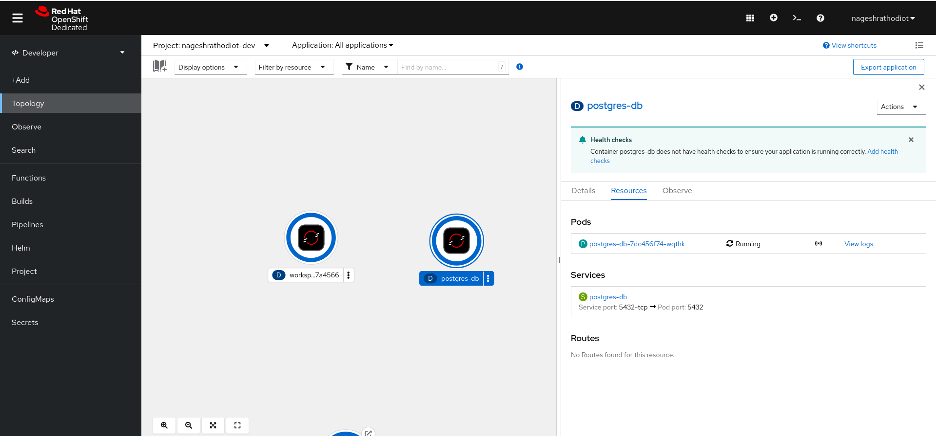
oc new-app --image=postgres --name=postgres-db -e POSTGRES_USER=admin -e POSTGRES_PASSWORD=redhat -e POSTGRES_DB=animal -e PGDATA=/var/lib/postgresql/data/pgdata1

After successfully deploying PostgreSQL, you will see the running pod in the Topology view in Developer perspective, as shown in Figure 5, below.

To store the image predictions in our project, we'll create a table named "animal" within the PostgreSQL database. This table will include a column named "prediction" to store the predicted class (e.g., "cat" or "dog").

Here's how to access the PostgreSQL console for interacting with the database.

• Click on the running pod.
• Select "View logs".
• Choose the "Terminal" option from tabs.

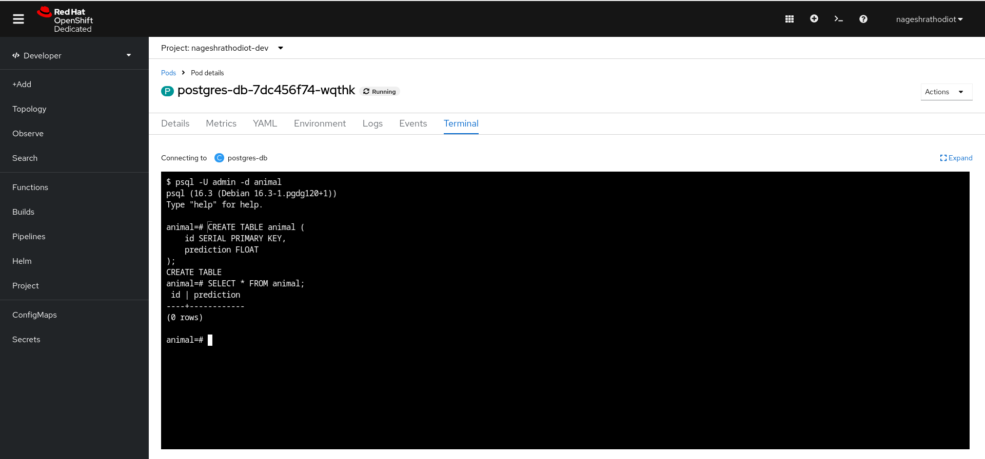
psql -U admin -d animal

To create tables and columns, use the following query:

CREATE TABLE animal (
 id SERIAL PRIMARY KEY,
    prediction FLOAT
);

Check the created table using the following query:

SELECT * FROM animal;

After executing the query, you will see the results on your pod terminal, as shown in Figure 6, below.

5. Consumer integration with database code

Merely having a consumer isn't sufficient to achieve real-time data processing. To accomplish this, we need to integrate prediction and database injection functionalities.

Replace the consumer code used in the previous step with the following code. Replace "Kafka_server_endpoint:9092" with your Kafka endpoint and "my-topic" with your Kafka topic name in the code below.

Replace "<postgresql-server>" with PostgreSQL endpoint.

The following code will wait for incoming data on the consumer side and subsequently execute image processing (image prediction) and database entry procedures:

! pip install kafka-python opencv-python psycopg2-binary
import numpy as np
from kafka import KafkaConsumer
import cv2
import psycopg2
consumer = KafkaConsumer("my-topic",bootstrap_servers=['Kafka_server_endpoint:9092'],
                       api_version=(0,10,1))
                       
# Function to process the image
def process_image(image):
   # Convert bytes to numpy array
   nparr = np.frombuffer(image, np.uint8)
   # Decode image
   img = cv2.imdecode(nparr, cv2.IMREAD_COLOR)
   # Reshape and resize
   img = cv2.resize(img, (256, 256))
   img = img.reshape((1,256,256,3))
   return img
   
def save_db(prediction):
   # Connect to PostgreSQL database
   conn = psycopg2.connect(
       dbname="animal",
       user="admin",
       password="redhat",
       host="<postgresql-server>",
       port="5432"
   )
   # Create a cursor
   cur = conn.cursor()
   try:
       # Execute the INSERT statement
       cur.execute("INSERT INTO animal (prediction) VALUES (%s)", (prediction,))
       # Commit the transaction
       conn.commit()
       print("Prediction saved to the database successfully!")
   except Exception as e:
       # Rollback the transaction if any error occurs
       conn.rollback()
       print("Error while saving prediction to the database:", e)
   finally:
       # Close the cursor and connection
       cur.close()
       conn.close()
       
for message in consumer:
   processed_image = process_image(message.value)
   prediction = model.predict(processed_image)
   save_db(float(prediction[0][0]))

On the consumer side, we handle and store the data in the database.

6. Test the end-to-end activity with the Kafka and prediction code base

Execute the consumer code now, ensuring it's positioned below the prediction codebase. Click on the "Execute" button. It will run in a loop, as shown in Figure 7, below.

7. Load the image from producer side 

It's time to execute the producer. Open the "Kafka_producer.ipynb" notebook. From the producer in this notebook, we will load an image of a dog. This image will simulate the live data streaming activity captured by the cameras.

Replace the producer code used in the previous step with the following code. Replace "Kafka_server_endpoint:9092" with your Kafka endpoint and "my-topic" with your Kafka topic name in the code below.

! pip install kafka-python opencv-python
import cv2
from kafka import KafkaProducer
producer=KafkaProducer(bootstrap_servers=['Kafka_server_endpoint:9092'],api_version=(0,10,1))
image = cv2.imread("dog.jpg")
ret, buffer = cv2.imencode('.jpg', image)
producer.send("my-topic",buffer.tobytes())

<kafka.producer.future.FutureRecordMetadata at 0x7f999d725640>

On the consumer side, you will receive confirmation logs, as shown in Figure 8.

Verifying prediction results in PostgreSQL

Once you've successfully executed the producer and consumer, it's crucial to confirm that the predicted classifications have been inserted into the database. Here's how to verify the results from a developer's perspective:

Accessing the PostgreSQL Console:

• Navigate to the OpenShift web console.
• Locate the pod corresponding to your PostgreSQL deployment configuration. This pod should be in a "Running" state.

Viewing Database Logs:

• Within the identified pod details, locate the section for logs.
• Select the option labeled "Terminal" to establish a terminal connection to the pod environment.

Executing SQL Queries:

• Once you have access to the terminal, log into the PostgreSQL database using the following command:

psql -U admin -d animal

• To check the entry from the image prediction, please use the following SQL query:

SELECT * FROM animal;

The complete code for image prediction is provided in this repository. You can simply clone this repository in Jupyter Notebook and add your "kaggle.json" file to it. Following that, you can execute the code.

Summary

This learning exercise explored real-time data processing using Apache Kafka (represented by AMQ Streams in this case). We learned to build a producer-consumer system that streams animal images, trains a machine learning model for image prediction, and stores the results in a PostgreSQL database. The exercise covered fetching the dataset, training the model, and integrating the prediction with data streaming.

Our goal is to make your data science projects successful, not just as experiments, but as part of the next generation of intelligent applications.