Network observability using TCP handshake round-trip time

In Red Hat OpenShift Container Platform (RHOCP), ensuring efficient packet delivery is paramount for maintaining seamless communication between applications. However, challenges like network congestion, misconfigured systems, or hardware limitations can lead to slow connections, impacting overall performance. Round-trip time (RTT), typically measured in milliseconds, plays a crucial role in monitoring network health and diagnosing issues.

Implementing smooth round-trip time (SRTT) with eBPF

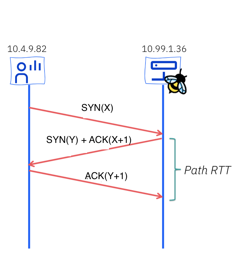
The RTT is the time it takes for a packet to travel from the sender to the receiver and back. In a network, RTT can vary due to factors like network congestion, varying route lengths, and other dynamic conditions. SRTT is introduced to provide a more consistent and less jittery representation of the RTT.

In Transmission Control Protocol (TCP), RTT is a crucial metric.

Our implementation leverages eBPF to register to fentry eBPF hook for tcp_rcv_established(). We extract the SRTT (smooth round-trip time) value from TCP sockets, correlating it to existing flows and enriching them with RTT values in nanoseconds.

When a new NetObserv flow is created and the RTT feature is enabled, an initial RTT of 10usec is assigned. This initial value for RTT may be considered quite low.

Upon triggering the eBPF socket, the flow RTT value is updated to reflect the maximum RTT value for that specific flow. See Figure 1.

For more detailed explanation of smoothed RTT estimation, refer to Karn's algorithm paper.

Why use fentry eBPF hook?

The eBPF fentry programs have lower overhead as they trigger the hook before calling the kernel function of interest.

In our implementation:

1. Register and link fentry hook for kernel's tcp_rcv_established()

   SEC("fentry/tcp_rcv_established")
   int BPF_PROG(tcp_rcv_fentry, struct sock *sk, struct sk_buff *skb) {
       if (sk == NULL || skb == NULL) {
           return 0;
       }
       return calculate_flow_rtt_tcp(sk, skb);
   }

2. Reconstruct the NetObserv flow key, including incoming interface Layer2, Layer3, and Layer4 info.

3. Match existing flows in the PerCPU hashmap flow table and enrich them with SRTT info from TCP sockets. If multiple SRTT values exist for the same flow, we take the maximum value.

Currently, our approach calculates RTT only for the TCP packets so flows, which are non-TCP, do not show RTT information.

Potential use cases

Flow RTT captured from eBPF flow_monitor hookpoints can serve various purposes.

• Network monitoring: Gain insights into TCP handshakes, helping network administrators identify unusual patterns, potential bottlenecks, or performance issues.

• Troubleshooting: Debug TCP-related issues by tracking latency and identifying misconfigurations.

How to enable RTT

To enable this feature, we need to create a FlowCollector object with the following fields enabled in eBPF config section as below.

apiVersion: flows.netobserv.io/v1beta2
kind: FlowCollector
metadata:
  name: cluster
spec:
  agent:
    type: eBPF
    ebpf:
      features:
        - FlowRTT

A quick tour of the UI

Once the FlowRTT feature is enabled, the RHOCP console plug-in automatically adapts to provide additional filter and show information across Netflow Traffic page views.

Open your RHOCP console and move to Administrator view -> Observe -> Network Traffic page as usual.

A new filter, Flow RTT is available in the common section. The FlowRTT filter will allow you to capture any flow that has an RTT more than a specific time in nanoseconds.

For production users, filtering on the TCP protocol, Ingress direction, and looking for FlowRTT values greater than 10,000,000 nanoseconds (10ms) can help identify TCP flows with high latency. This filtering approach allows users to focus on specific network flows that may be experiencing significant delays. By setting a threshold of 10ms, you can efficiently isolate and address potential latency issues in your TCP traffic.

Overview

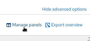
New graphs are introduced in the Advanced options -> Manage panels popup (Figure 2).

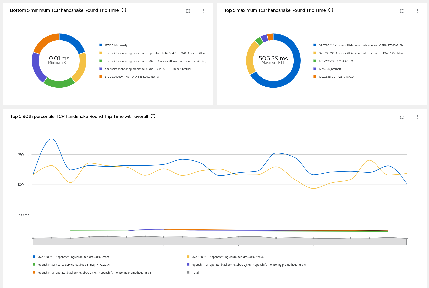
• Top X average TCP handshake round-trip time with overall (donut or lines)
• Bottom X minimum TCP handshake round-trip time with overall (donut or lines)
• Top X maximum TCP handshake round-trip time with overall (donut or lines)
• Top X 90th percentile TCP handshake round-trip time with overall (donut or lines)
• Top X 99th percentile TCP handshake round-trip time with overall (donut or lines)

These two graphs (see Figure 3) can help you to identify the slowest TCP flows and their trends over time. Use the filters to drill down into specific pods, namespaces, or nodes.

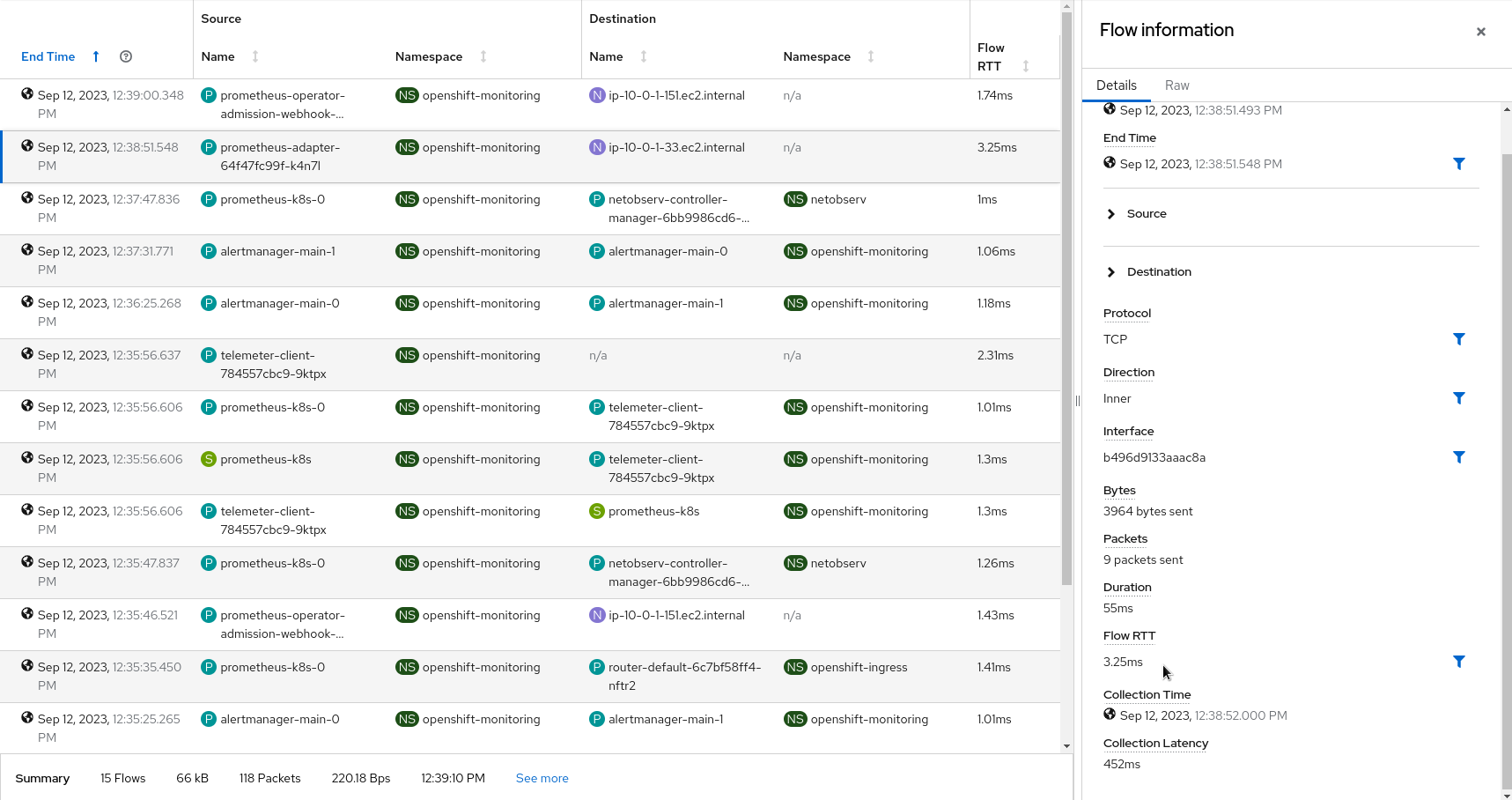
Traffic flows

The table view (Figure 4) shows the Flow RTT in both column and side panel.

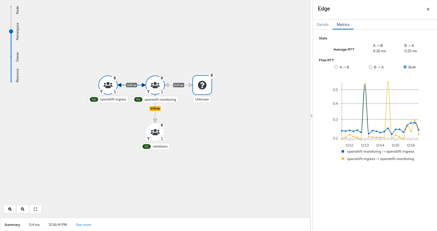
Topology

Last but not least, the topology view displays min / max / avg / p90 / p99 RTT latency on edges. Clicking on a node or an edge will allow you to see per direction metrics and the related graph. See Figure 5.

Future improvements

Here is a non-exhaustive list of future improvements coming for a full featured round-trip time analysis:

• Latest RTT in Topology view
• Prometheus metrics and alerting

Feedback

We hope you liked this article!

NetObserv is an open source project available on GitHub. Feel free to share your ideas, use cases, or ask the community for help.