The performance of your Apache Kafka environment will be affected by many factors, including choices, such as the number of partitions, number of replicas, producer acknowledgments, and message batch sizes you provision. But different applications have different requirements. Some prioritize latency over throughput, and some do the opposite. Similarly, some applications put a premium on durability, whereas others care more about availability. This article introduces a way of thinking about the tradeoffs and how to design your message flows using a model I call the Kafka optimization theorem.
Optimization goals for Kafka
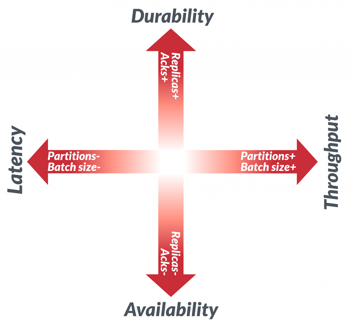
Like other systems that handle large amounts of data, Kafka balances the opposing goals of latency and throughput. Latency, in this article, refers to how long it takes to process a single message, whereas throughput refers to how many messages can be processed during a typical time period. Architectural choices that improve one goal tend to degrade the other, so they can be seen as opposite ends of a spectrum.
Two other opposed goals are durability and availability. Durability (which in our context also includes consistency) determines how robust the entire system is in the face of failure, whereas availability determines how likely it is to be running. There are tradeoffs between these two goals as well.
Thus, the main performance considerations for Kafka can be represented as in Figure 1. The diagram consists of two axes, each with one of the goals at one of its ends. For each axis, performance lies somewhere between the two ends.
Kafka priorities and the CAP theorem
The CAP theorem, which balances consistency (C), availability (A), and partition tolerance (P), is one of the foundational theorems in distributed systems.
Note: The word partition in CAP is totally different from its use in Kafka streaming. In CAP, a partition is a rupture in the network that causes two communicating peers to be temporarily unable to communicate. In Kafka, a partition is simply a division of data to permit parallelism.
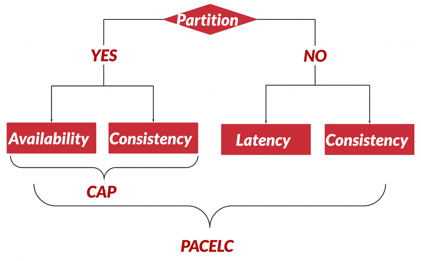
Partition tolerance in the CAP sense is always required (because one can't guarantee that a partition won't happen), so the only real choice in CAP is whether to prioritize CP or AP.
But CAP is sometimes extended with other considerations. In the absence of a partition, one can ask what else (E) happens and choose between optimizing for latency (L) or consistency (C). The complete list of considerations is called PACELC (Figure 2). PACELC explains how some systems such as Amazon's Dynamo favor availability and lower latency over consistency, whereas ACID-compliant systems favor consistency over availability or lower latency.
Kafka primitives
Every time you configure a Kafka cluster, create a topic, or configure a producer or a consumer, you are making a choice of latency versus throughput and of availability versus durability. To explain why, we have to look into the main primitives in Kafka and the role that client applications play in an event flow.
Partitions
Topic partitions represent the unit of parallelism in Kafka, and are shown on the horizontal axis in Figure 1. In the broker and the clients, reads and writes to different partitions can be done fully in parallel. While many factors can limit throughput, a higher number of partitions for a topic generally enables higher throughput, and a smaller number leads to lower throughput.
However, a very large number of partitions causes the creation of more metadata that needs to be passed and processed across all brokers and clients. This increased metadata can degrade end-to-end latency unless more resources are added to the brokers. This is a somewhat simplified description of how partitions work on Kafka, but it will serve to demonstrate the main tradeoff that the number of partitions leads to in our context.
Replicas
Replicas determine the number of copies (including the leader) for each topic partition in a cluster, and are shown on the vertical axis in Figure 1. Data durability is ensured by placing replicas of a partition in different brokers. A higher number of replicas ensures that the data is copied to more brokers and offers better durability of data in the case of broker failure. On the other hand, a lower number of replicas reduces data durability, but in certain circumstances can increase availability to the producers or consumers by tolerating more broker failures.
Availability for a consumer is determined by the availability of in-sync replicas, whereas availability for a producer is determined by the minimum number of in-sync replicas (min.isr). With a low number of replicas, the availability of overall data flow depends on which brokers fail (whether it's the one with the partition's leader of interest) and whether the other brokers are in sync. For our purposes, we can assume that fewer replicas lead to higher application availability and lower data durability.
Producers and consumers
Partitions and replicas represent the broker side of the picture, but are not the only primitives that influence the tradeoffs between throughput and latency and between durability and availability. Other participants that shape the main Kafka optimization tradeoffs are found in the client applications.
Topics are used by producers that send messages and consumers that read these messages. Producers and consumers also state their preference between throughput versus latency and durability versus availability through various configuration options. It is the combination of topic and client application configurations (and other cluster-level configurations, such as leader election) that defines what your application is optimized for.
Consider the flow of events consisting of a producer, a consumer, and a topic. Optimizing such an event flow for average latency on the client side requires tuning the producer and consumer to exchange smaller batches of messages. The same flow can be tuned for average throughput by configuring the producer and consumer for larger batches of messages.
Producers and consumers involved in a message flow also state their preference for durability or availability. A producer that favors durability over availability can demand a higher number of acknowledgments by specifying acks=all. A lower number of acknowledgments (lower than the default min.isr, which means 0 or 1) could lead to higher availability from the producer point of view by tolerating a higher number of broker failures. However, this lower number reduces data durability in the case of catastrophic events affecting the brokers.
The consumer configurations influencing the vertical dimension are not as straightforward as the producer configurations, but depend on the consumer application logic. A consumer can favor higher consistency by committing message consumption offsets more often or even individually. This does not affect the durability of the records in the broker, but does affect how consumed records are tracked, and can prevent duplicate message processing in the cosumer. Alternatively, the consumer can favor availability by increasing various timeouts and tolerating broker failures for longer periods of time.
The Kafka optimization theorem
We have defined the main actors involved in an event flow as a producer, a consumer, and a topic. We've also defined the opposing goals we have to optimize for: throughput versus latency and durability versus availability. Given these parameters, the Kafka optimization theorem states that any Kafka data flow makes the tradeoffs shown in Figure 3 in throughput versus latency and durability versus availability.
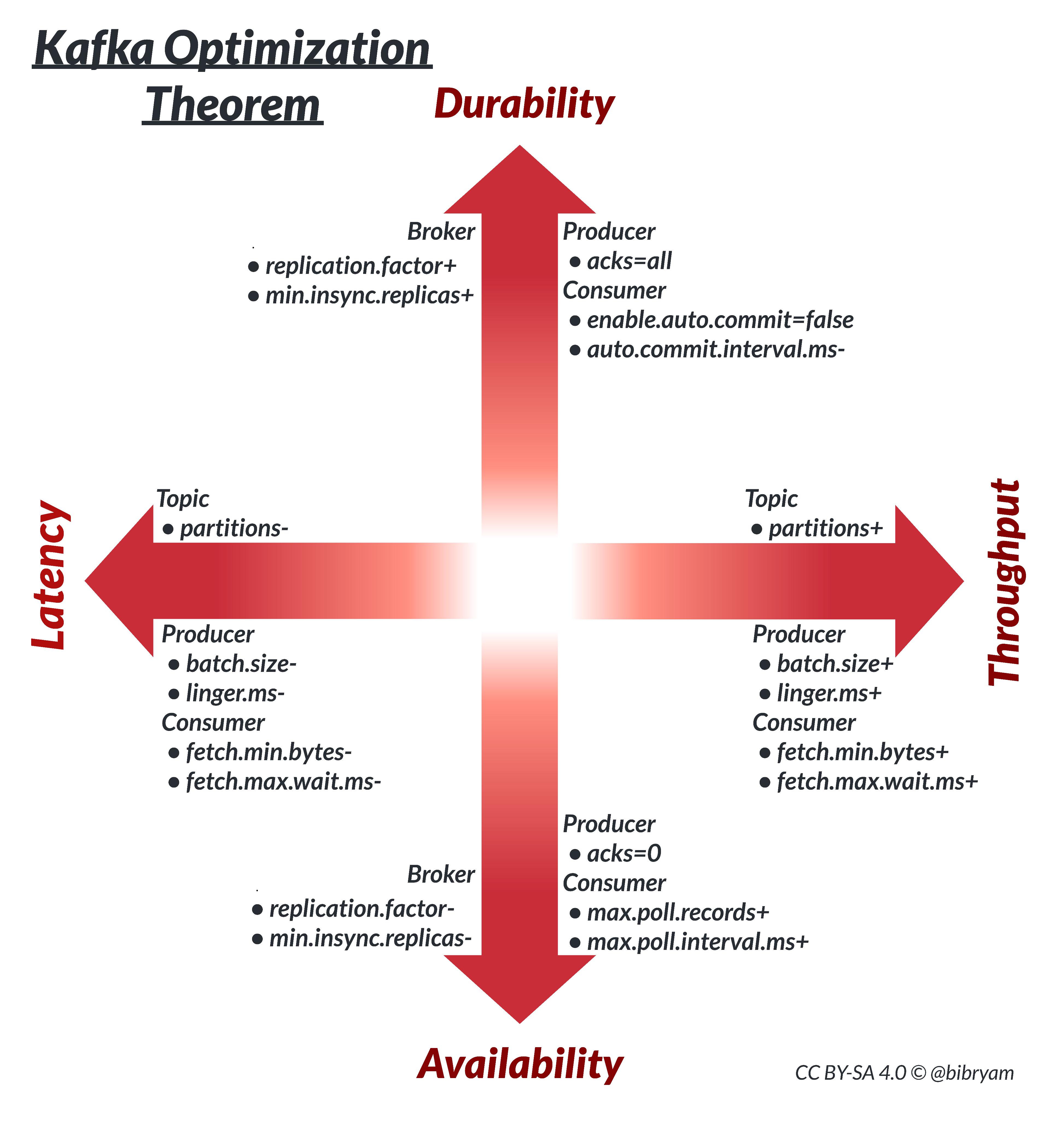
The Kafka optimization theorem and the primary configuration options
For simplicity, we put producer and consumer preferences on the same axes as topic replicas and partitions in Figure 3. Optimizing for a particular goal is easier when these primitives are aligned. For example, optimizing an end-to-end data flow for low latency is best achieved with smaller producer and consumer message batches combined with a small number of partitions.
A data flow optimized for higher throughput would have larger producer and consumer message batches and a higher number of partitions for parallel processing. A data flow optimized for durability would have a higher number of replicas and require a higher number of producer acknowledgments and granular consumer commits. A data flow that is optimized for availability would prefer a smaller number of replicas and a smaller number of producer acknowledgments with larger timeouts.
In practice, there is no correlation in the configuration of partitions, replicas, producers, and consumers. It is possible to have a large number of replicas for a topic (min.isr), but have a producer that requires a 0 or 1 for acknowledgments. Or you could configure a higher number of partitions because your application logic requires it, and small producer and consumer message batches. These are valid scenarios in Kafka, and one of its strengths is that it's a highly configurable and flexible eventing system that satisfies many use cases.
Nevertheless, the framework proposed here can serve as a mental model for the main Kafka primitives and how they relate to the optimization dimensions. If you understand the foundational forces, you can tune them in ways specific to your application and understand the effects.
The golden ratio
The proposed Kafka optimization theorem deliberately avoids stating numbers, instead just laying out the relationships between the main primitives and the direction of change. The theorem is not intended to serve as a concrete optimization configuration but rather as a guide that shows how reducing or increasing a primitive configuration influences the direction of the optimization. Yet sharing a few of the most common configuration options accepted as the industry best practices could be useful as a starting point and demonstration of the theorem in practice.
Kafka clusters today, whether run on-premises with something like Strimzi, or as a fully managed service offering such as OpenShift Streams for Apache Kafka, are almost always deployed within a single region. A production-grade Kafka cluster is typically spread into three availability zones with a replication factor of 3 (RF=3) and minimum in-sync replicas of 2 (min.isr=2).
These values ensure a good level of data durability during happy times, and good availability for client applications during temporary disruptions. This configuration represents a solid middle ground, because specifying min.isr=3 would prevent producers from producing even when a single broker is affected, and specifying min.isr=1 would affect both producer and consumer when a leader is down. Typically, this replication configuration is accompanied by acks=all on the producer side and by default offset commit configurations for the consumers.
While there are commonalities in consistency and availability tradeoffs among different applications, throughput and latency requirements vary. The number of partitions for a topic is influenced by the shape of the data, the data processing logic, and its ordering requirements. At the same time, the number of partitions dictates the maximum parallelism and message throughput you can achieve. As a consequence, there is no good default number or range for the partition count.
By default, Kafka clients are optimized for low latency. We can observe that from the default producer values (batch.size=16384, linger.ms=0, compression.type=none) and the default consumer values (fetch.min.bytes=1, fetch.max.wait.ms=500). The producer prior to Kafka 3 had acks=1, which recently changed to acks=all to create a preference for durability rather than availability or low latency. Optimizing the client applications for throughput would require increasing wait times and batch sizes five to tenfold and examining the results. Knowing the default values and what they are optimized for is a good starting point for your service optimization goals.
Summary
CAP is a great theorem for failure scenarios. While failures are a given and partitioning will always happen, we have to optimize applications for happy paths too. This article introduces a simplified model explaining how Kafka primitives can be used for performance optimization.
The article deliberately focuses on the main primitives and selective configuration options to demonstrate its principles. In real life, more factors influence your application performance metrics. Encryption, compression, and memory allocation affect latency and throughput. Transactions, exactly-one semantics, retries, message flushes, and leader election affect consistency and availability. You might have broker primitives (replicas and partitions) and client primitives (batch sizes and acknowledgments) optimized for competing tradeoffs.
Finding the ideal Kafka configuration for your application will require experimentation, and the Kafka optimization theorem will guide you in the journey.
Last updated: October 9, 2023