Optimize model serving at the edge with RawDeployment mode

The edge environment presents multiple challenges. Beyond the typical network connectivity limitations, there are other drawbacks to consider. As computing moves closer to the edge, the environment becomes more constrained. AI/ML processes often demand significant computational power and specialized hardware, which can be difficult to provide in an environment with limited space and resources. Additionally, edge locations often lack extensive dedicated IT support, requiring operations with minimal human intervention. 

On the positive side, bringing AI to the edge means that models are trained, managed, and served closer to where the data is generated. This introduces several advantages, such as keeping data within the local environment and faster decision-making while reducing dependency on network connectivity.

The model serving component within Red Hat OpenShift AI allows serving models using various platforms. For large models, single-model serving is the ideal option, as it enables the allocation of independent resources for each model. This platform, based on KServe, offers two deployment modes: Serverless and RawDeployment.

RawDeployment is more focused on edge environments as it does not rely on service mesh, saving valuable resources and providing several advantages like full control over Kubernetes resources, enabling detailed customization of deployments. Taking all this into account, we have chosen this serving mode for our scenario.

In this article, you will learn how to set up Red Hat OpenShift AI on single node OpenShift to make use of RawDeployment model serving to expose an AI model capable of predicting the amount of rainfall based on exogenous data.

Red Hat OpenShift AI configuration

This journey starts from an empty single node OpenShift cluster at the edge. We chose single node OpenShift because it's a lighter OpenShift solution with a single master-worker node, making it ideal for environments with limited resources. This node will be used to develop, train, and serve an AI model straight to our device fleet at the far edge. 

The first step is to install and configure Red Hat OpenShift AI on our single node OpenShift. OpenShift AI brings together various machine learning capabilities on a single platform and will be used for both training and serving the model. 

Now, let's see how to install the operator.

1. Open the OpenShift web console, and navigate to the Operators tab on the left panel. Then select OperatorHub.
2. Type OpenShift AI to search the component in the operators’ catalog (Figure 1).

3. Select the Red Hat OpenShift AI operator and click Install. Make sure that the selected Version is 2.16.0 onwards. 
4. The operator will be deployed in the redhat-ods-operator namespace. Review the rest of the parameters and press Install to start the operator installation.
5. When the installation finishes, we need to configure the DataScienceCluster custom resource. Select Create DataScienceCluster.
6. Once in the configuration page, scroll down and click Components. Here you can see a list of all the components that can be enabled/disabled from Red Hat OpenShift AI.
7. Locate and select the kserve component to configure it. Unless otherwise specified, the default deployment mode used by KServe is Serverless. Change the defaultDeploymentMode to RawDeployment and verify that the managementState shows Managed.
8. Also, under serving, we need to modify the stack used for model serving. RawDeployment mode does not use Knative. Therefore, we need to switch the managementState to Removed. The configuration should look like Figure 2.

9. Keep the rest of the default values and press Create.
10. Because KServe RawDeployment mode does not require a service mesh for network traffic management, we can also disable Red Hat OpenShift Service Mesh. To do so, navigate to the DSC Initialization tab within our operator.
11. In the DSC Initialization tab, you will see the DSCI resource created during the operator installation. Select default-dsci.
12. Click on the YAML tab in the details page to modify the resource definition.
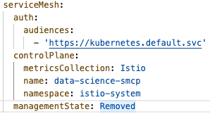
13. Locate the serviceMesh component and change the managementState field to Removed (Figure 3). Then click Save.

14. The DSCInitialization resource will change its status to Ready.

Now you should be able to access the OpenShift AI web console. On the right side of the top navigation bar, you will find a square icon made up of nine smaller squares. Click it and select Red Hat OpenShift AI from the drop-down menu (Figure 4).

A new tab will open. Log in again using your OpenShift credentials and you will be redirected to the Red Hat OpenShift AI landing page. There, create a new Data Science Project.

Configure object storage

Red Hat OpenShift AI requires an S3-compatible object storage to save the new trained models and to be able to serve them. If you already have access to an S3-compatible object store, feel free to jump to the next section. Otherwise, you can follow the upcoming procedure to deploy the MinIO object storage system in your single node OpenShift.

1. Open your OpenShift web console and create a new namespace called minio.
2. In the upper-right corner, next to the squared icon we used to access the OpenShift AI dashboard, there is a plus (+) button that allows us to create resources from a YAML. 
3. Make sure to select the Project: minio from the drop-down menu at the top.
4. Copy and paste the contents of this minio.yaml file. It defines a persistent volume, a secret with the MinIO access credentials, the deployment itself, and a couple of services and routes to expose the MinIO console. 
5. Finally, to create all the components mentioned, press the blue Create button.
6. To access the MinIO console, open the Networking section on the left menu and select Routes.

7. Locate the minio-ui route and click on the URL in the Location column. The route should look similar to this one:

   https://minio-ui-minio.apps.sno.redhat.com

8. You will be redirected to the MinIO logging page. Use the following credentials to access the dashboard:
   • User: minio
   • Password: minio123
9. The last step will be creating a bucket. An S3 bucket is similar to a folder in a file system where we can store any object. Press Create a bucket.
10. Complete the Bucket Name field with the desired folder name (I named mine storage, as shown in Figure 5). Then click on Create Bucket.

At this point, we can use the S3 bucket to store data. In order to make it accessible from our Jupyter environment, we need to create a DataConnection in our node, indicating the set of s3 configuration values. These steps will be explained in the next section. 

Create a DataConnection

Red Hat OpenShift AI creates DataConnection resources as OpenShift secrets. Those secrets store all the configuration values that facilitate connecting data science projects to object storage buckets. Those buckets can contain either the dataset used for the training or the AI models to be served. Let’s configure the DataConnection.

1. Open again the Red Hat OpenShift AI web console and navigate to the Connections tab (Figure 6). There, select Create connection.
2. In the new pop-up window, complete the following fields:
   • Connection type: Select S3 compatible object storage - v1.
   • Name: Name for the secret. I’m using storage.
   • Access key: Username defined when deploying MinIO. Ours was minio.
   • Secret key: Add the MinIO password. In our case, minio123.
   • Endpoint: You can get the API endpoint URL from the MinIo service in OCP. Yours should be: http://minio-service.minio.svc.cluster.local:9000.
   • Region: It doesn’t really matter here. The default value is us-east-1.
   • Bucket: As we saw, I created the storage folder to store my trained model.
3. When completed, select Add data connection.

A new Secret called aws-connection-storage will be created containing all the specified values stored in base64 format.

Create a Workbench

A workbench is a containerized workspace that operates within a pod and contains a collection of different AI/ML libraries and a JupyterLab server. Click on the Workbenches tab and select Create workbench. Complete the form depending on your use case specifications:

• Name: Type your preferred name. I will use training.
• Image selection: The election will depend on your model requirements. Click on View package information to see the packages included. I will use Pytorch.
• Version selection: The recommendation is to use the latest package version.
• Container size: Select it according to your hardware limitations: number of CPUs, memory, and request capacity of the container.
• Accelerator: If your node has a graphical card, you can select it from here to speed up the model training.
• Number of accelerators: Select as many graphic cards as available in your node.
• Check the Create new persistent storage box.
  • Name: Type any desired name for the persistent volume.
  • Persistent storage size: Specify the desired capacity for the volume.
• Select Attach existing connections and verify that the storage connection is selected. 

Review your configuration and press Create workbench. This last step will trigger the workbench creation. Wait until the Status shows Running and click Open.

Training and saving our Model

We can use Jupyter Notebooks to train the AI model we want. You can either import an existing notebook or create a new one from scratch. Figure 7 shows an example notebook, in which I train a very simple AI model capable of predicting the amount of rainfall based on the exogenous data coming from external sensors. You can use it as a reference to build and train your own model. You can find the notebooks in this Git repo.

The chart displays historical rainfall data alongside the values of sensors measured each day. As you can see, the data has been split after 2005. The data from the beginning of the historical series up to that point will be used to train the model, while the data from 2005 to the end will be used for validation.

After collecting the dataset, it's time to train our Forecast model.

Looking at the graph in Figure 8, we can compare the real validation data (red line) with the trend predicted by the model (orange line). As we can see, the model has been able to learn from the training data and correctly identifies the trends.

Once we have our new model, we need to save it in the S3 bucket so it can be served later. To do so, create another notebook like the one shown in Figure 9.

When you finish running all the cells, you will have saved the trained model in your MinIO bucket, ready to be consumed.

Create a model serving platform

The ultimate goal of model serving is to make a model available as a service that can be accessed through an API. In the case of deploying large AI models, OpenShift AI includes a single model serving platform that pulls the model from the S3 bucket, and creates the inference endpoints on the data science projects to allow applications to send inference requests.

1. In the Red Hat OpenShift AI dashboard, navigate to the Models tab inside our project.
2. Locate the Single-model serving platform option and select Deploy model.
3. Complete the following fields in the form:
   • Model name: Type the name for the model server. I will use Forecast.
   • Serving runtime: There are different runtimes to choose. Select the one that suits best your model. As an example, I will use the OpenVINO Model Server.
   • Model framework: Select the format in which you saved the model. My model was exposed in onnx-1 format.
   • Model server replicas: Choose the number of pods to serve the model.
   • Model server size: Assign resources to the server. 
   • Accelerator: If there are GPUs available on your node, you can select them here.
   • Check the Existing data connection box, if it is not already selected.
     • Name: Click on your DataConnection. Remember, ours was named storage.
     • Path: Indicate the path to your model location in the S3 bucket. That’s: models/forecast/. We don't need to specify the full path because KServe will automatically pull the model from the /1/ subdirectory in the path specified.
4. When configured, click on Deploy.

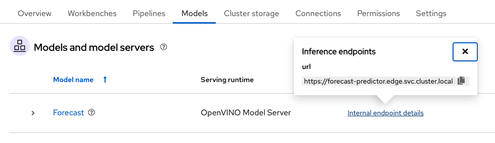
At that moment, new ServingRuntime and InferenceService resources will be created in your node. In the Models tab, your new Model Service should appear. Wait until you see a green checkmark in the Status column. Also, the Inference endpoint field (Figure 10) will show you the model inference API to make requests to.

Querying our model

As a result, the model is available as a service and can be accessed using API requests. The Inference endpoint enables you to interact with the model and return predictions based on data inputs. Here is an example of how to make a RESTful inference request to a machine learning model hosted in a model server:

curl -ks <inference_endpoint_url>/v2/models/<model_name>/infer -d '{ "model_name": "<model_name>", "inputs": [{ "name": "<name_of_model_input>", "shape": [<shape>], "datatype": "<data_type>", "data": [<data>] }]}' -H 'Authorization: Bearer <token>'

There, you just need to specify the inference endpoint we got from the Model Server and the name of the model. Finally, specify the new data values to be sent to the model so they can be used for prediction. 

If you want to know more about how to use inference endpoints to query models, check the official documentation.

Conclusion

This article provided a step-by-step guide to deploying and serving AI models at the edge using Red Hat OpenShift AI on a single node OpenShift cluster. It covered setting up OpenShift AI, configuring object storage with MinIO, creating data connections, training and saving a model in a Jupyter workbench, and finally deploying and querying the model using KServe's RawDeployment mode. This approach enables efficient AI/ML workloads in resource-constrained environments by leveraging edge computing capabilities and reducing reliance on centralized infrastructure.

To learn more about OpenShift AI, visit the OpenShift AI product page or try our hands-on learning paths.