RHEL AI in action: Streamline AI workflows with RAG, LAB, and RAGLAB

Anaconda setup

For each experiment, it's important to create a dedicated environment using Anaconda. This setup helps with package management and ensures isolation, minimizing the risk of dependency conflicts across different projects.

Follow the steps below:

1. Go to Anaconda Downloads and copy the link to the 64-Bit (x86) Installer (1007.9M):

   curl -O https://repo.anaconda.com/archive/Anaconda3-2024.06-1-Linux-x86_64.sh

2. Install Anaconda:

       bash Anaconda3-2024.06-1-Linux-x86_64.sh # accept the TnC

3. Create and activate a new Anaconda environment:

       conda create -n mcs-rhelai-milvus-dev python=3.11 anaconda
       conda activate mcs-rhelai-milvus-dev

4. Run a Jupyter notebook with port forwarding:

      pip install jupyter
      #run jupyter lab
      jupyter lab  --no-browser --ip 0.0.0.0 --port=8080

5. Open Jupyter notebook in browser open terminal in your local machine and use the below command to connect:

      ssh -L 8080:localhost:8080 cloud-user@10.31.124.12

First approach: RAG (granite-7b-redhat-lab + Milvus Lite)

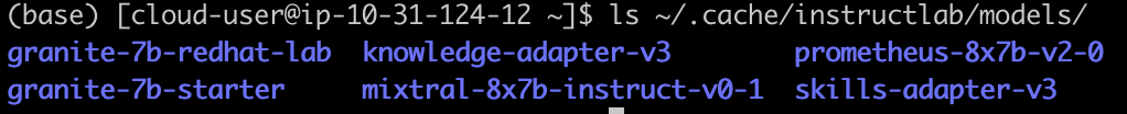
We started by implementing a retrieval-augmented generation (RAG) approach, utilizing the granite-7b-redhat-lab model. This pre-trained large language model (LLM) can be easily downloaded using the InstructLab command:

ilab model download --repository docker://<repository_and_model> --release <release>

(Refer to the official doc for more details on this command.) 

Figure 1 shows the path to the downloaded models.

Next, we set up Milvus Lite, a lightweight vector database, to store document embeddings. We used the LangChain Milvus wrapper to simplify the integration process. To install Milvus, use simple a pip command:

pip install -qU langchain_milvus

The following steps outline how we ingested the data into Milvus and utilized it for retrieval during the RAG process.

Step 1: Import required packages and download embeddings

We began by importing the necessary packages and downloading the our chosen embeddings:

from langchain_milvus import Milvus
from langchain_community.embeddings import HuggingFaceEmbeddings 

URI = "./milvus_example.db"
embeddings = HuggingFaceEmbeddings(model_name="mixedbread-ai/mxbai-embed-large-v1")

Step 2: Load documents

We used DirectoryLoader from LangChain to load documents into the system. There are various methods to achieve this, but in this case, we chose to load documents from a local directory:

from langchain_community.document_loaders import DirectoryLoader 

loader = DirectoryLoader('../data/')
documents = loader.load()
// Optionally, split the documents into smaller chunks

Step 3: Add documents to Milvus

Once the documents were loaded, we converted them into embeddings and stored them in Milvus:

vector_store_saved = Milvus.from_documents(
    documents, embeddings, 
    collection_name="milvus_mcs", 
    connection_args={"uri": URI}
)

The vector embeddings are stored locally, as illustrated in Figure 2. In our case, they were saved in the file milvus_example.db, which allows for efficient retrieval during the RAG process.

Set up the RAG pipeline

After ingesting the data, the next step is to configure the RAG pipeline by connecting the granite-7b-redhat-lab model to the retrieval system. This involves querying Milvus for relevant document embeddings and integrating the retrieved information with the LLM’s response generation.

To do this, the granite-7b-redhat-lab model needs to be hosted and running in RHEL AI. This can be easily achieved using the following InstructLab command:

ilab model serve --model-path ~/.cache/instructlab/models/granite-7b-redhat-lab/

By default, the model is served on 127.0.0.1:8000. Once the model is up and running, you will notice GPU resources being utilized for processing. Figure 3 shows GPU resource being consumed.

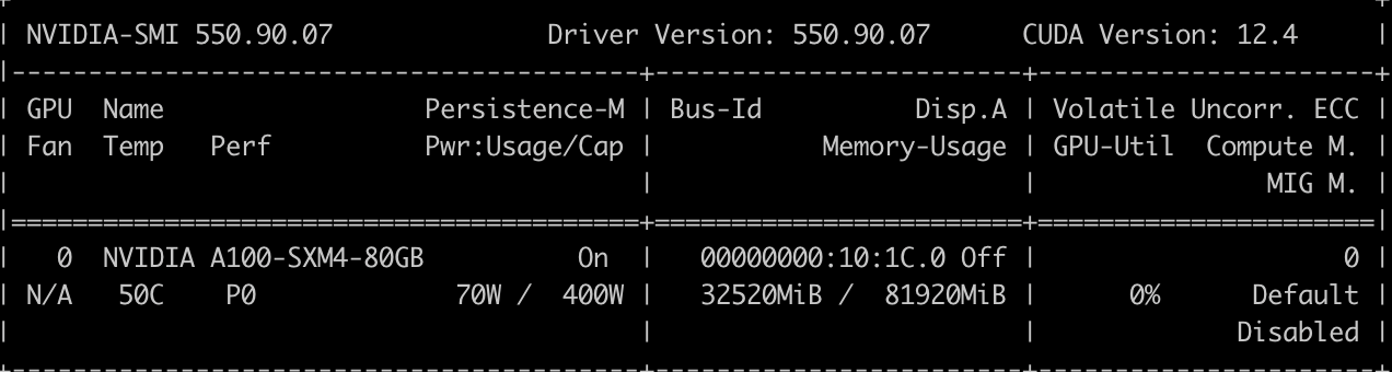
For more details on model serving, refer to the documentation.

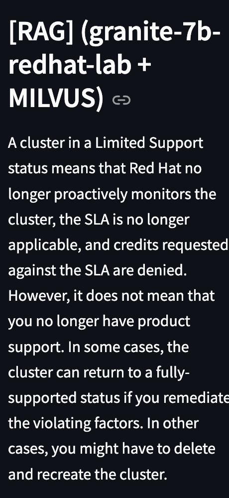
We have implemented a basic Streamlit app to demonstrate this setup. Figures 4 and 5 show the RAG approach with the Streamlit app.

Second approach: Fine-tuning the granite-starter model

Fine-tuning an LLM allows for adapting the model to specific tasks or datasets, improving its accuracy and relevance. In our case, fine-tuning the granite-starter model helps enhance the performance of a question-answer chatbot based on domain-specific  knowledge. We use the qna.yaml file and knowledge documents, as outlined in the data pre-processing section, to fine-tune the model. Once the data is validated, the following steps are carried out.

Step 1: Create a synthetic dataset using sample examples

To generate additional training data, we create a synthetic dataset using MCS-based examples. This is achieved by running the following InstructLab command:

ilab data generate

This command runs the synthetic data generation (SDG) process using the mixtral-8x7B-instruct model as the teacher to generate synthetic data.

Since this process can be time-consuming and depends on the volume of data, it is recommended to run the InstructLab commands within a tmux session to maintain continuity. To create a new tmux session, run:

tmux new -s session_name

For our sample set, the SDG process took approximately 10.5 hours and produced around 70,000 new samples.

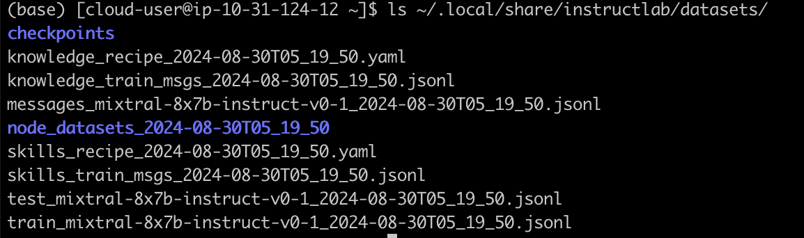
To count the number of generated samples, you can use the following command:

wc -l ~/.local/share/instructlab/datasets/checkpoints/<your_data_file>/*.jsonl

After the SDG process completes, verify that the new files are created as expected. The new dataset created using SDG process is shown in Figure 6.

Step 2: Training

RHEL AI utilizes your taxonomy tree and synthetic data to create a newly trained model that incorporates your domain-specific knowledge and skills through a multi-phase training and evaluation process.

For training, we focus on two essential files:

• <knowledge-train-messages-file>
• <skills-train-messages-file>

The training process is initiated using the following InstructLab command:

ilab model train --strategy lab-multiphase \
   --phased-phase1-data ~/.local/share/instructlab/datasets/knowledge_train_msgs_2024-08-30T05_19_50.jsonl \
   --phased-phase2-data ~/.local/share/instructlab/datasets/skills_train_msgs_2024-08-30T05_19_50.jsonl

It is advisable to run the above commands in the tmux session created earlier.

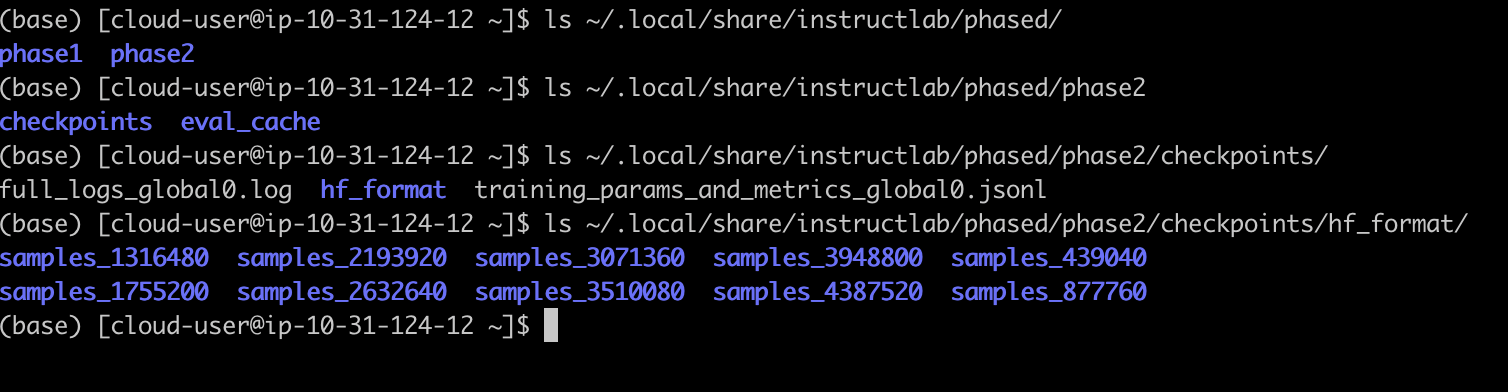
Figure 7 shows the new checkpoints created.

Step 3: Serve and chat with the model

To interact with your newly trained model, you need to activate it on a machine by serving the model. The ilab model serve command initiates a vLLM server, allowing you to chat with the model.

For our use case, the best-performing model selected was samples_4387520. RHEL AI evaluates all checkpoints from phase 2 of model training using the Multi-turn Benchmark (MT-Bench) and identifies the best-performing checkpoint as the fully trained output model. You can serve this model with the following command:

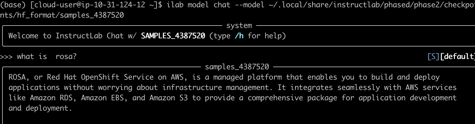
ilab model serve --model-path ~/.local/share/instructlab/phased/phase2/checkpoints/hf_format/samples_4387520

Once the model is being served, open another terminal to start chatting with the fine-tuned model using the command:

ilab model chat --model ~/.local/share/instructlab/phased/phase2/checkpoints/hf_format/samples_4387520

With these steps, your fine-tuned granite-7b model is now ready for interaction. Figure 8 shows fine-tuned model interaction using ilab chat command.

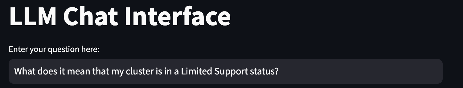
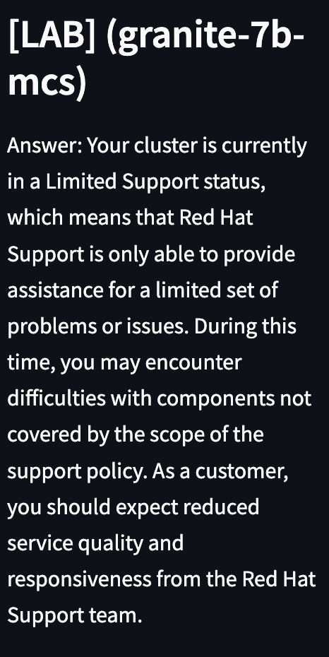
Let’s test its capabilities using our Streamlit application. Figure 9 shows fine-tuned model interaction on the Streamlit application, and Figure 10 shows the model's answer.

Third approach: RAGLAB (RAG leveraging iLAB)

This hybrid approach enhances the model’s ability to generate more accurate and contextually relevant responses, particularly for domain-specific tasks. In this phase, we combine our fine-tuned granite-7b model with the RAG approach.

This approach closely resembles Approach 1; however, instead of utilizing a pre-trained model, we leverage a domain-specific model. Based on the results from our experiments (currently conducted manually), we are confident that RAGLAB provides a robust solution to meet our requirements. 

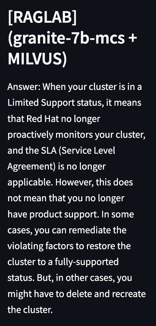
Figure 11 shows RAGLAB approach in action. Figure 12 shows the model's answer to the user query.

To enhance scalability and performance for larger datasets, users can consider transitioning from Milvus Lite to Enterprise Milvus (e.g., WxD Milvus) to better accommodate their specific use cases.

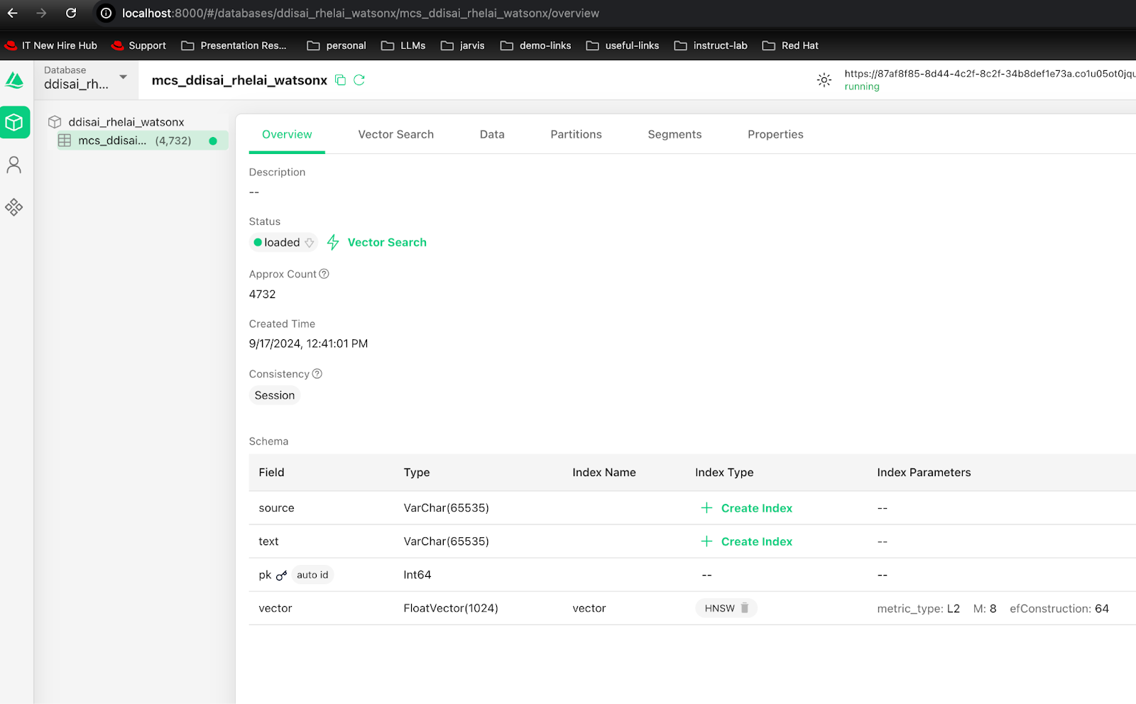
Connecting to Watsonx Milvus follows the same procedure as with Milvus Lite, with the key difference being the use of a database URL, username, and password instead of localhost. We can employ tools like Attu to verify our ingested data.  Figure 13 shows stored vector embeddings that can be viewed using tools like Attu.

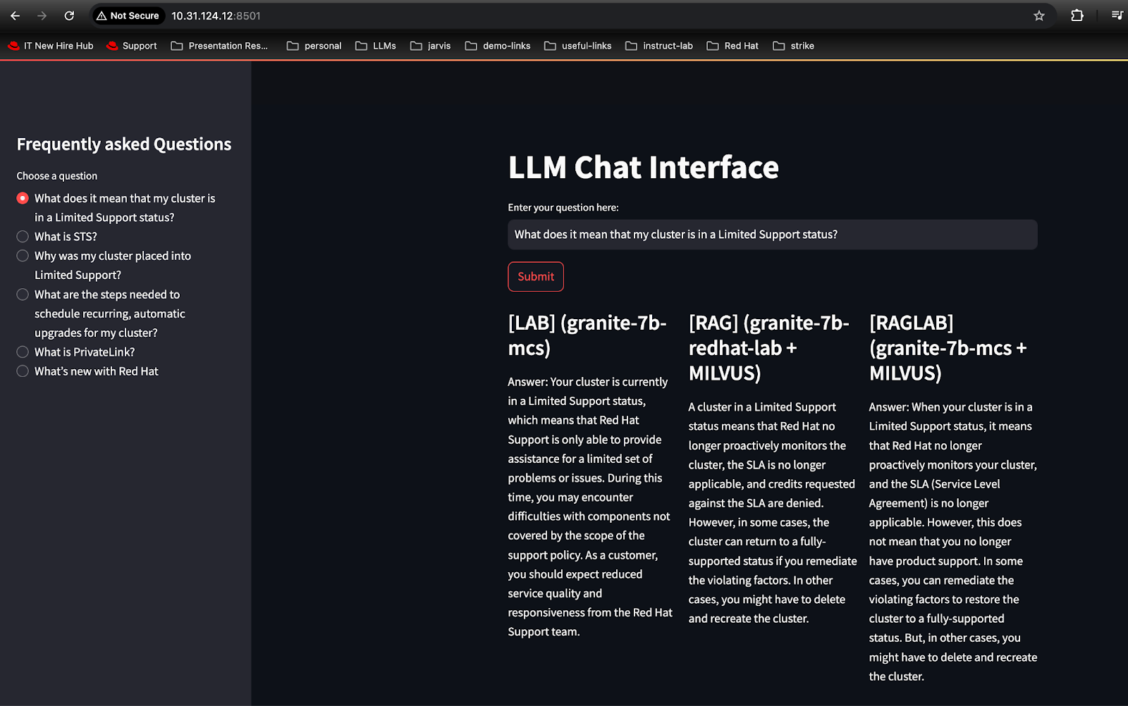
The remaining processes remain unchanged from those discussed in the previous approaches. We will now utilize our Streamlit app to showcase comparisons across all three approaches, as shown in Figure 14.

Conclusion

This article demonstrated how you can apply Red Hat Enterprise Linux AI (RHEL AI) for fine-tuning Granite LLM models using three key approaches: retrieval-augmented generation (RAG), direct model fine-tuning (LAB), and an integrated method with RAGLAB. We highlighted essential steps including data preprocessing, environment setup, and the use of Milvus as a vector database to efficiently store and query embeddings. This comprehensive framework enables building and deploying scalable AI solutions, such as a chatbot application, leveraging a seamless end-to-end pipeline.