Recently, I was working on an edge computing demo that uses machine learning (ML) to detect anomalies at a manufacturing site. This demo is part of the AI/ML Industrial Edge Solution Blueprint announced last year. As stated in the documentation on GitHub, the blueprint enables declarative specifications that can be organized in layers and that define all the components used within an edge reference architecture, such as hardware, software, management tools, and tooling.
At the beginning of the project, I had only a general understanding of machine learning and lacked the practitioner's knowledge to do something useful with it. Similarly, I’d heard of Jupyter notebooks but didn’t really know what they were or how to use one.
This article is geared toward developers who want to understand machine learning and how to carry it out with a Jupyter notebook. You'll learn about Jupyter notebooks by building a machine learning model to detect anomalies in the vibration data for pumps used in a factory. An example notebook will be used to explain the notebook concepts and workflow. There are plenty of great resources available if you want to learn how to build ML models.
What is a Jupyter notebook?
Computation notebooks have been used as electronic lab notebooks to document procedures, data, calculations, and findings. Jupyter notebooks provide an interactive computational environment for developing data science applications.
Jupyter notebooks combine software code, computational output, explanatory text, and rich content in a single document. Notebooks allow in-browser editing and execution of code and display computation results. A notebook is saved with an .ipynb extension. The Jupyter Notebook project supports dozens of programming languages, its name reflecting support for Julia (Ju), Python (Py), and R.
You can try a notebook by using a public sandbox or enabling your own server like JupyterHub. JupyterHub serves notebooks for multiple users. It spawns, manages, and proxies multiple instances of the single-user Jupyter notebook server. In this article, JupyterHub will be running on Kubernetes.
The Jupyter notebook dashboard
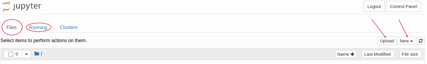
When the notebook server first starts, it opens a new browser tab showing the notebook dashboard. The dashboard serves as a homepage for your notebooks. Its main purpose is to display the portion of the filesystem accessible by the user and to provide an overview of the running kernels, terminals, and parallel clusters. Figure 1 shows a notebook dashboard.
The following sections describe the components of the notebooks dashboard.
Files tab
The Files tab provides a view of the filesystem accessible by the user. This view is typically rooted to the directory in which the notebook server was started.
Adding a notebook
A new notebook can be created by clicking the New button or uploaded by clicking the Upload button.
Running tab
The Running tab displays the currently running notebooks known to the server.
Working with Jupyter notebooks
When a notebook is opened, a new browser tab is created that presents the notebook's user interface. Components of the interface are described in the following sections.
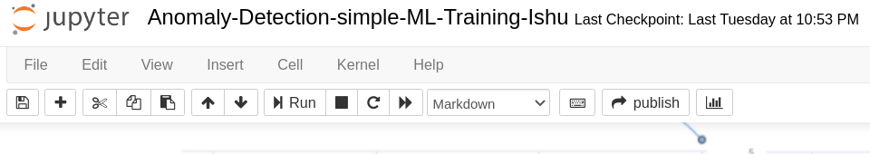
Header
At the top of the notebook document is a header that contains the notebook title, a menu bar, and a toolbar, as shown in Figure 2.
Body
The body of a notebook is composed of cells. Cells can be included in any order and edited at will. The contents of the cells fall under the following types:
- Markdown cells: These contain text with markdown formatting, explaining the code or containing other rich media content.
- Code cells: These contain the executable code.
- Raw cells: These are used when text needs to be included in raw form, without execution or transformation.
Users can read the markdown and text cells and run the code cells. Figure 3 shows examples of cells.

Editing and executing a cell
The notebook user interface is modal. This means that the keyboard behaves differently depending on what mode the notebook is in. A notebook has two modes: edit and command.
When a cell is in edit mode, it has a green cell border and shows a prompt in the editor area, as shown in Figure 4. In this mode, you can type into the cell, like a normal text editor.

When a cell is in command mode, it has a blue cell border, as shown in Figure 5. In this mode, you can use keyboard shortcuts to perform notebook and cell actions. For example, pressing Shift+Enter in command mode executes the current cell.

Running code cells
To run a code cell:
- Click anywhere inside the [ ] area at the top left of a code cell. This will bring the cell into command mode.
- Press Shift+Enter or choose Cell—>Run.
Code cells are run in order; that is, each code cell runs only after all the code cells preceding it have run.
Getting started with Jupyter notebooks
The Jupyter Notebook project supports many programming languages. We’ll use IPython in this example. It uses the same syntax as Python but provides a more interactive experience. You’ll need the following Python libraries to do the mathematical computations needed for machine learning:
- NumPy: For creating and manipulating vectors and matrices.
- Pandas: For analyzing data and for data wrangling or munging. Pandas takes data such as a CSV file or a database, and creates from it a Python object called a
DataFrame. ADataFrameis the central data structure in the Pandas API and is similar to a spreadsheet as follows:- A
DataFramestores data in cells. - A
DataFramehas named columns (usually) and numbered rows.
- A
- Matplotlib: For visualizing data.
- Sklern: For supervised and unsupervised learning. This library provides various tools for model fitting, data preprocessing, model selection, and model evaluation. It has built-in machine learning algorithms and models called estimators. Each estimator can be fitted to some data using its
fitmethod.
Using a Jupyter notebook for machine learning
We’ll be using the MANUela ML model as a notebook example to explore various components needed for machine learning. The data used to train the model is located in the raw-data.csv file.
The notebook follows the workflow shown in Figure 6. An explanation of the steps follows.

Step 1: Explore raw data
Use a code cell to import the required Python libraries. Then, convert the raw data file (raw-data.csv) to a DataFrame with a time series, an ID for the pump, a vibration value, and a label indicating an anomaly. The required Python code is shown in a code cell in Figure 7.

Running the cell produces a DataFrame with raw data, shown in Figure 8.

Now visualize the DataFrame. The upper graph in Figure 9 shows a subset of the vibration data. The lower graph shows manually labeled data with anomalies (1 = anomaly, 0 = normal). These are the anomalies that the machine learning model should detect.

Before it can be analyzed, the raw data needs to be transformed, cleaned, and structured into other formats more suitable for analysis. This process is called data wrangling or data munging.
We’ll be converting the raw time series data into small episodes that can be used for supervised learning. The code is shown in Figure 10.

We want to convert the data to a new DataFrame with episodes of length 5. Figure 11 shows a sample time series data set.

If we convert our sample data into episodes with length = 5, we get results similar to Figure 12.

Let’s now convert our time series data into the episodes, using the code in Figure 13.

Figure 13: Converting data into episodes.
Figure 14 explores the data with episodes of length 5 and the label in the last column.

Figure 14: Episodes of length 5 and the label in the last column.
Note: In Figure 14, column F5 is the latest data value, where column F1 is the oldest data for a given episode. The label L indicates whether there is an anomaly.
The data is now ready for supervised learning.
Step 2: Feature and target columns
Like many machine learning libraries, Sklern requires separated feature (X) and target (Y) columns. So Figure 15 splits our data into feature and target columns.

Figure 15: Splitting data into feature and target columns.
Step 3: Training and testing data sets
It’s a good practice to divide your data set into two subsets: One to train a model and the other to test the trained model.
Our goal is to create a model that generalizes well to new data. Our test set will serve as a proxy for new data. We’ll split the data set into 67% for the training sets and 33% for the test set, as shown in Figure 16.

Figure 16: Splitting data into training and test data sets.
We can see that the anomaly rate for both training and test sets is similar; that is, the data set is pretty fairly divided.
Step 4: Model training
We will perform model training with a DecisionTreeClassifier. Decision Trees is a supervised learning method used for classification and regression. The goal is to create a model that predicts the value of a target variable by learning simple decision rules inferred from the data features.
DecisionTreeClassifier is a class that performs multi-class classification on a dataset, although in this example we’ll be using it for classification into a single class. DecisionTreeClassifier takes as input two arrays: An array X as features and an array Y as labels. After being fitted, the model can then be used to predict the labels for the test data set. Figure 17 shows our code.

Figure 17: Model training with DecisionTreeClassifier.
We can see that the model achieves a high accuracy score.
Step 5: Save the model
Save the model and load it again to validate that it works, as shown in Figure 18.

Figure 18: Saving the model.
Step 6: Inference with the model
Now that we've created the machine learning model, we can use it for inference on real-time data.
In this example, we’ll be using Seldon to serve the model. For our model to run under Seldon, we need to create a class that has a predict method. The predict method can receive a NumPy array X and return the result of the prediction as:
- A NumPy array
- A list of values
- A byte string
Our code is shown in Figure 19.

Figure 19: Using Seldon to serve the machine learning model.
Finally, let’s test whether the model can predict anomalies for a list of values, as shown in Figure 20.

Figure 20: Inference using the model.
We can see that the model achieves a high score for inference, as well.
References for this article
See the following sources for more about the topics discussed in this article:
Last updated: August 15, 2022