Oversaturation is a sneaky problem that wastes time, money, and costly GPU cycles when benchmarking large language models (LLMs). In Reduce LLM benchmarking costs with oversaturation detection, we established what oversaturation is and explained why oversaturation detection (OSD) is crucial for controlling our LLM benchmarking budgets.
Now, we're moving from the problem to the solution. But how do you teach a machine to spot a condition that is difficult to even define? Here's how we built the algorithm.
Our goal: Don't waste money
Our goal is simple, but it has two conflicting parts:
- Catch a "bad" (oversaturated) run. This is a true alert. Every minute we let a "bad" run continue, we are literally burning money on a premium GPU for useless results.
- Never stop a "good" (undersaturated) run. This is a false alert, and in many ways, it's even worse. We're just invalidating a perfectly good, expensive test, leaving a permanent "hole" in our benchmark and forcing us to run the entire test all over again.
This creates a high-stakes balancing act. Our algorithm needs to be aggressive enough to catch bad runs, but not so aggressive that it kills good ones.
The problem of "when": Survival analysis
The core challenge—"How long until an event happens?"—belongs to a specific field of data science called survival analysis. It started in medicine but is used everywhere from engineering to business. Our specific questions were:
- "How long will this good run survive before our algorithm mistakenly stops it?"
- "How long will this bad run survive before our algorithm correctly catches it?"
A standard metric from this field is the concordance index (C-Index), which measures if our algorithm "makes sense" by checking if "bad" runs were stopped before "good" runs.
The "1 second versus 1 hour" flaw
Consider two scenarios:
- Scenario A: Our algorithm raises a true alert (catches saturation) after 1 minute, but raises a false alert (stops a good run) after 2 minutes.
- Scenario B: Our algorithm raises a true alert after 1 second, but raises a false alert after 1 hour.
The standard C-Index treats both scenarios as equally perfect because it only cares about the order. However, for our business goal, Scenario B is definitely better. It saves us an entire hour of wasted GPU time. We needed a metric that rewarded the magnitude of the time gap, not just the correct order.
Our solution: The Soft-C-Index
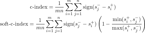
Because no standard metric fit our needs, we built our own: the Soft-C-Index. The Soft-C-Index measures the percentage of "effective" time, not just the correct order. It adds a "soft" component that heavily rewards algorithms for creating a wider gap between catching bad runs early and stopping good ones late.
The standard C-Index uses a "hard" sign function, while our Soft-C-Index adds a "softness" factor that measures the magnitude of the time difference (Figure 1).
The real "Aha!" moment comes from these next two graphs (Figures 2 and 3). We ran a simulation where our algorithm got progressively "smarter," creating a wider time gap between true alerts and false alerts.
This is the key. The Soft-C-Index curve keeps climbing, correctly reflecting that we are saving more money. It's aligned with our business goal: saving GPU minutes.
Our evaluation method
Okay, we've invented our metric. Now we need a test environment. Our evaluation method has three key steps:
- Get labeled data: Manually label 500+ of our reports as "good" or "bad."
- Handle "unraised" cases: Figure out what to do when an algorithm never fires an alert.
- Fix biased data: Solve a nasty "cheating" problem we found in our dataset.
Step 1: Labeling the data
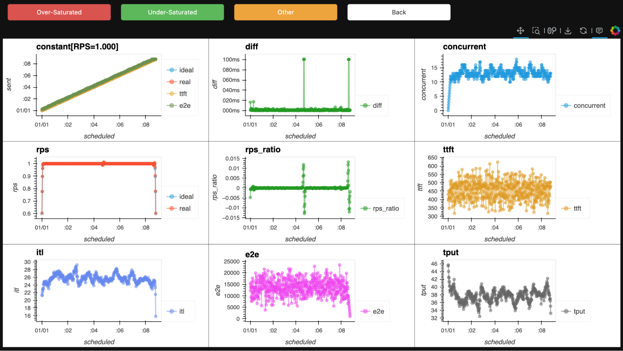
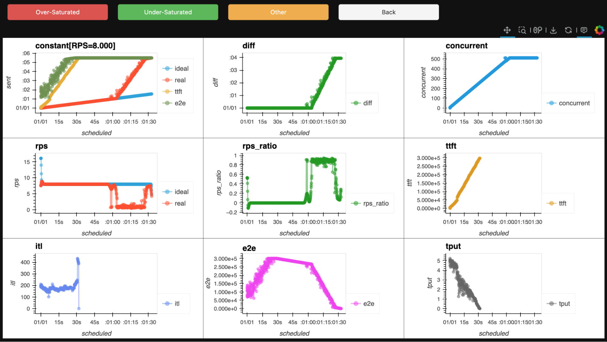
We started with more than 500 of our benchmark reports, which our experts reviewed one by one, manually labeling them as either undersaturated (good) or oversaturated (bad). How could they tell? By looking at the charts. See Figures 4 and 5.
Step 2: Handling "unraised" cases
We had to figure out what to do with "unraised" cases, or when our algorithm runs and never raises an alert. We settled on a "best-case"/"worst-case" inference system:
- If the run was good and our algorithm never alerted: This is a perfect outcome, a best-case scenario.
- If the run was bad and our algorithm never alerted: This is a total failure, a worst-case scenario.
This logic allows us to calculate soft_c_index_best, soft_c_index_worst, and soft_c_index_avg, which is the main metric we use.
Step 3: Fixing the biased data
Our dataset was heavily biased: most high-load (high RPS) runs were oversaturated, and most low-load runs were undersaturated. This allowed our algorithm to learn how to read the "load" setting, which is cheating.
To compensate, we duplicated the data to make the load look higher. We ran three scenarios: 1) duplicated the data once, 2) twice, and 3) eight times. To demonstrate this, we used a "bad" algorithm (a simple threshold) and a "good" algorithm and evaluated them on our augmented dataset. The following table shows the soft_c_index_avg score.
| Algorithm | Multiplier=1 | Multiplier=2 | Multiplier=8 |
|---|---|---|---|
| my-bad-algorithm | 0.706 | 0.805 | 0.548 |
| my-good-algorithm | 0.821 | 0.830 | 0.812 |
The "bad" algorithm's performance rapidly deteriorates as the average load shifts. The "good" algorithm, in contrast, is better in every aspect. Its score is high, and it's almost completely multiplier invariant, meaning it's stable and reliable. Now we have a complete evaluation setup.
Next steps
In this blog, we went through the technical details of choosing an evaluation metric (Soft-C-Index), labeling our dataset, and fixing bias with data augmentation. In the third and final part of this series, we'll walk through the algorithm exploration itself, show our iterative error analysis, and reveal the discovery process of our best algorithm so far.
Read part 3: Building a oversaturation detector with iterative error analysis
Last updated: November 24, 2025