Build, train, and run your TensorFlow model

To really dive into AI, you need to use one of the many frameworks provided for these tasks. TensorFlow, a machine learning library from Google, is the most well-known and widely used framework to do this kind of work. It has several layers, allowing you to get as deep into the weeds as you need when writing code for machine learning.

For the purposes of this tutorial, we will stay at a fairly high level, using the packaged Keras library. Keras lets you look at neural networks in terms of layers of nodes and is generally easy for new users to use. The library doesn't require a lot of the advanced math that some lower layers might need. Instead, Keras requires just a general understanding of when to apply certain techniques.

In this learning path, we will use Keras to work on the MNIST data set. Although it is possible for non-AI code to do things such as classifying handwritten digits classification, AI is currently state of the art for such loosely defined tasks. AI also has the secondary benefit of being significantly easier to program in some cases. Some other approaches involve decision trees or support vector machines.

The sections that you will be working through include:

1. Reloading the data and creating DataFrames for testing and training
2. Creating model features and labels
3. Creating a TensorFlow model with several convolution layers
   1. Conv2D
   2. MaxPooling2D
   3. Flatten
   4. Dense
   5. Dropout
   6. Dense with softmax activation
4. Compiling the model
5. Training the model
6. Testing the model
7. Saving the model
8. Running the model

Reloading the data and creating DataFrames for testing and training

Open the 02-MNIST-Tensorflow.ipynb notebook. This notebook covers some of the data preparation required, as well as training the model and evaluating the model.

Because this is a new notebook, you need to load the TensorFlow data again, as shown in Figure 16.

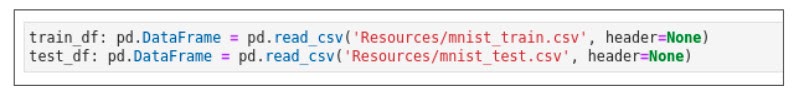
You are now ready to create model features and labels.

Creating models and features

After you create the DataFrames, split the data set in the same way, separating the features from the labels using the following Python code:

train_features: np.ndarray = train_df.loc[:, 1:].values

Next, you need to unpack the features you extracted into a four-dimensional data structure. This is necessary because of the AI we will be using later in the notebook. The AI will have a convolutional layer. We'll explore this layer in more detail in the sections that follow. However, to use it, we need to format the data in the way the machine learning methods expect. The convolutional layer expects each input to be a three-dimensional array containing a set of pixels arranged by width and height. Then, each element in that matrix must be an array of one to three elements. Our data set is all greyscale, so we'll have a single element in each array, But images could also be represented as a set of three elements representing an [R, G, B] pixel value.

In our case, we simply reshape our features into 60,000 28x28x1 arrays using the following Python code:

train_features = train_features.reshape((train_features.shape[0], 28, 28, 1))

Next, you need to normalize the data. This is a very important step for two reasons: First, it helps the model learn faster when the inputs are in the range [0, 1], and second, it helps prevent a problem known as vanishing/exploding gradients in certain neural networks

To normalize the data, simply divide it by the maximum value: 255 in our case, because we know that the data is in the range [0, 255].

train_features = train_features / 255.0

Finally, split out the labels using the following Python code:

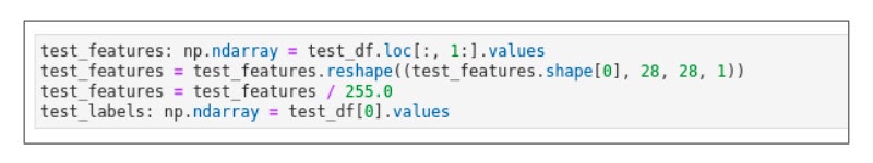
train_labels: np.ndarray = train_df[0].values

Repeat the same preprocessing for the test dataset.

It's important to understand why we have a separate dataset for training and testing. Neural networks are designed to "learn" associations in data by looking at large sets of data. However, it can also teach some bad habits. For example, if all of the digits were written by someone right-handed, the algorithm may learn habits associated with right-handed writing and perform poorly for digits written with the left hand. This learning of peculiarities of a given sample of data is called overfitting. The problem arises whenever a training dataset doesn't fully accurately reflect reality.

One good way to help avoid good overfitting is to ensure that the algorithm performs well on data it hasn't seen before. To do this, we separate some of the data into a test data set (Figure 17) that is used only to evaluate the performance of the AI after the model was trained on other data. This is only one tool for keeping AI accurate. Bias and overfitting can occur in many ways, but it's always good practice to evaluate the AI test data set to ensure it isn't overfitted to the training data set.

You can read some more about bias in AI in many online articles, but this MIT article summarizes some of the problems well.

Now you finally create your model using the following Python code:

model: tf.keras.models.Sequential = tf.keras.models.Sequential()

This model is sequential, meaning that each layer sends its outputs to all inputs of the following layer.

We will add several layers into this model, and I'll explain why these certain layers are good to use when solving certain problems. However, many combinations could work. You need to build good intuition about when and how to use certain types of AI to ensure that your AI models perform well.

Create a TensorFlow model with several convolution layers

We are now ready to take a look at convolution. We'll cover the following types of convolution:

• Conv2D
• MaxPooling2D
• Flatten
• Dense
• Dropout
• Dense (with softmax activation)

Convolution (Conv2D)

Convolution is one of the most important techniques in modern AI. It's built on top of Fourier transformations, and it is currently the state of the art when it comes to image analysis. In a basic convolution, one takes a small snapshot of the pixels, examines how they blend together, and applies a filter to strengthen or weaken the effect. This is done over the entire image, allowing edges to be strengthened or unimportant parts of the image to be blurred.

A deeper understanding of this layer requires quite a bit of math, but an excellent analysis can be found in this primer.

Because this is the first layer, we also can specify input_shape to help TensorFlow understand the shape of the input. Use the following Python code to add a layer performing convolution over a two-dimensional input:

model.add(tf.keras.layers.Conv2D(filters=32, kernel_size=(3, 3), input_shape=(28, 28, 1)))

MaxPooling2D

Next, we define a layer pooling the maximum value in a two-dimensional grid. This algorithm is called MaxPooling2D. It allows a larger image to be downsampled by the maximum value in a given grid. In our previous layer, we modified the image to emphasize the important parts of the image (edges, spaces, etc.). To make the image easier to process, we take small grids (2x2 in this case), find the maximum value inside that grid, and pass that value on to the next layer. This helps eliminate less important data from the image and makes processing faster and usually more precise. The Python code we use for MaxPooling2D is:

model.add(tf.keras.layers.MaxPooling2D(pool_size=(2, 2), strides=2))

Flatten

Now we will flatten the multidimensional output into a single-dimensional output. This layer is pretty simple, flattening our two-dimensional grid into a single array. The action helps the next layer process the data more efficiently. The Dense layer that follows works best with one-dimensional or two-dimensional inputs to keep the underlying matrix multiplications simple. The Dense layer can understand the same associations as in arrays of more dimensions because the images are all flattened according to the same algorithm. The Python code we use to flatten is:

model.add(tf.keras.layers.Flatten())

Dense

Having flattened the images, we will now create a densely-connected classification layer.

Dense layers are the basic classification layers. They receive inputs and determine which parts of the input are important when classifying data. A dense layer makes its decisions through something called an activation function. The activation function is based on observations of the human brain and how one neuron activates another. Certain signal levels in a neuron affect how large an electrical impulse is sent out to connected neurons. These neurons take a weighted sum of the inputs and produce an output. In AI, a comparable process updates the weights as part of an optimization function that we'll cover a bit later with techniques like gradient descent and backpropagation.

To learn more about activation functions (a very key concept) and how they work, have a look at this article.

The Python code we use for a densely-connected classification layer is:

model.add(tf.keras.layers.Dense(units=64, activation=tf.nn.relu))

Dropout

Next, we want to remove certain dense nodes from the training data set to prevent overfitting. We use Dropout to accomplish this.

Overfitting was defined earlier in this learning path. To prevent AI from learning too many of the exact peculiarities of the data set, there are several techniques broadly referred to as regularization. This is one technique that is easy to apply to Keras layers. The dropout layer randomly removes a certain percentage of the previous layers from the network while training, to prevent them from becoming too specialized to the training data set.

You can read more about regularization techniques in this article.

The Python code we use for removing dense nodes (Dropout) is:

model.add(tf.keras.layers.Dropout(rate=0.2))

Dense with softmax activation

We now are ready for a classifier layer that outputs a maximum value. This is accomplished using a Dense algorithm with softmax activation.

This final, output layer classifies the work done by all the previous layers. To do so, we take a layer that has nodes representing each class and take the maximum activation value. That is to say, whichever set of neurons from the previous network provided the greatest confidence in its class becomes the output. In the case of a 0, we would see node 0 having the highest "activation" across all of the neurons. In cases where the comparison close, such as having a .59 and .60 activation, we still take the maximum, knowing that there will likely be some misclassifications in edge cases like that.

For some fun reading about misclassification based on close levels of activation, check out this article. This article covers a set of issues related to misclassifying dogs and bagels (and a web search of this problem can reveal more fun instances of similar issues).

The Python code we use for adding a classifier layer that outputs a maximum value is:

model.add(tf.keras.layers.Dense(10, activation=tf.nn.softmax))

Compile the model

Finally, we are ready to compile our model using an optimizer and loss function.

Our optimizer is the function or set of functions that determine how the model updates its weights as it trains. The loss function calculates the accuracy of a result from training. This loss function is minimized by using the optimization function.

The techniques used to train the model are called (broadly) gradient descent and backpropagation. Essentially, the optimizer updates the weights, performs a training iteration, and then updates the weights to be more accurate based on how much they contributed to the correct or incorrect classification during training. Backpropagation refers to how the optimizer calculates the degree that each neuron contributes to the answer. The specific functions used can heavily affect how well the model performs at a given task. In this case, we use the Adam optimizer and the SparseCategoricalCrossentropy function to calculate the loss.

The metric we want to print out as we go through the training and testing is accuracy. We defined this in the previous notebook as:

???????? = ???????_??????????? / ?????_???????????

Explanations of optimization, loss, and gradient descent tend to be somewhat mathematical. Rather than dive in further in this notebook, you can read about how these algorithms are calculated in this article.

The adam optimizer is a variant of Stochastic Gradient Descent and has some benefits that you can read about in this article.

The loss functions are explained in this article.

The Python code we use to compile our model, using our chosen optimizer and loss function, is:

model.compile(optimizer='adam',

              loss='sparse_categorical_crossentropy',

              metrics=['accuracy'])

A model.summary() method in Figure 18 shows a summary of the layers and how they are connected.

Train the model

We are now ready to train our model, using the features and labels we formatted earlier. Depending on the machine, training can happen very quickly or very slowly. Training a model in some more advanced cases could even take days, explaining why the advancements in GPU performance have been so crucial in bringing AI into viability for solving many problems that were once thought intractable. We train the model using the following Python code:

model.fit(train_features, train_labels, epochs=3)

We expect that the accuracy will increase with each epoch we use (Figure 19).

Test the model

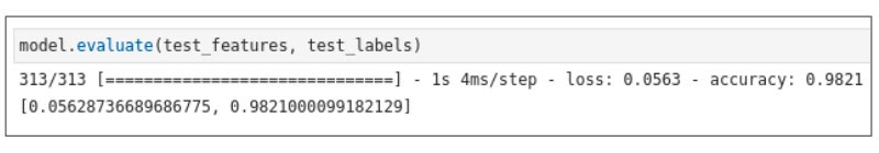
Now that we have trained our model and feel confident with its accuracy, we are ready to test the model. Testing is critical to ensure that the model will generalize to data it hasn't seen before. In this case, we want the accuracy and loss to be fairly close to the values we saw at the end of the training. If they're not, our model is probably overfitted to the training data to some extent and won't perform well on data it hasn't seen before.

Note that no AI is perfect, and this is a departure from traditional computer science, where results tend to be either right or wrong. This tradeoff is important to understand and is why AI is not suitable for every problem. However, AI is becoming more practical as it has opened up the ability to solve many problems that were once considered nearly intractable.

We test the model using the following Python code and observe that the model accuracy is 0.9821 and model loss is 0.0563 (Figure 20). These results are very good!

Save the model

Finally, we want to save our model out to storage because we'll reuse the model in a later notebook.

There are many formats in which one can save the model, but the most common are:

• HDF5, which saves the model as a single file including the configuration of the layers and weights.
• JSON, which saves just the configuration of the layers. This choice requires the weights to be saved separately.
• SavedModel, a TensorFlow-specific layout involving a few directories. This format is required by the TensorFlow Serving server, which allows you to easily serve the model to other systems.

The following Python code saves the model in HDF5 format

model.save('mnist-model/mnist-model.h5', overwrite=True, include_optimizer=True)

Run the model

Now let's run the model and see whether it can correctly classify an image of a digit. Figure 21 shows a "handwritten" number 9. The model correctly predicts the digit and assigns the label 9.

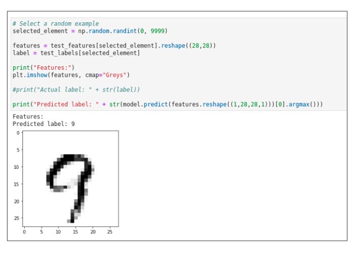
Congratulations! Your model can take the image of a digit and correctly classify it by outputting the correct digit. This concludes the TensorFlow learning path.

Interested in learning more? Explore Red Hat OpenShift Data Science in the Developer Sandbox for Red Hat OpenShift.