The Apache Kafka project includes a Streams Domain-Specific Language (DSL) built on top of the lower-level Stream Processor API. This DSL provides developers with simple abstractions for performing data processing operations. However, how one builds a stream processing pipeline in a containerized environment with Kafka isn’t clear. This second article in a two-part series uses the basics from the previous article to build an example application using Red Hat AMQ Streams.
Now let's create a multi-stage pipeline operating on real-world data and consume and visualize the data.
The system architecture
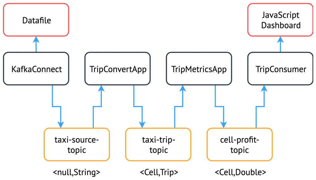
In this article, we build a solution that follows the architecture diagram below. It may be worth referring back here for each new component:
The dataset and problem
The data we chose for this example is the New York City taxi journey information from 2013, which was used for the ACM Distributed Event-Based Systems (DEBS) Grand Challenge in 2015. You can find a description of the data source here.
This example's dataset is provided as a CSV file, with the columns detailed below:
| Column | Description |
|---|---|
| medallion | an md5sum of the identifier of the taxi - vehicle bound |
| hack_license | an md5sum of the identifier for the taxi license |
| pickup_datetime | time when the passenger(s) were picked up |
| dropoff_datetime | time when the passenger(s) were dropped off |
| trip_time_in_secs | duration of the trip |
| trip_distance | trip distance in miles |
| pickup_longitude | longitude coordinate of the pickup location |
| pickup_latitude | latitude coordinate of the pickup location |
| dropoff_longitude | longitude coordinate of the drop-off location |
| dropoff_latitude | latitude coordinate of the drop-off location |
| payment_type | the payment method - credit card or cash |
| fare_amount | fare amount in dollars |
| surcharge | surcharge in dollars |
| mta_tax | tax in dollars |
| tip_amount | tip in dollars |
| tolls_amount | bridge and tunnel tolls in dollars |
| total_amount | total paid amount in dollars |
Source: DEBS 2015 Grand Challenge.
We can explore interesting avenues within this dataset, such as following specific taxis to calculate:
- The money earned from one taxi throughout the course of a day.
- The distance from the last drop-off to the next pick-up to find out whether they travel far without a passenger.
- The average speed of the taxi's trip by using the distance and time; we then use the pick-up and drop-off coordinates to guess the amount of traffic encountered.
The example
The processing we chose for this example is relatively straightforward. We calculate the total amount of money (fare_amount + tip_amount) earned within a particular area of the city, based off of journeys starting there. This calculation involves splitting the input data into a grid of different cells and then summing the total amount of money taken for every journey that originates from any cell. To accomplish this, we have to consider splitting up processing in a way that ensures that our output is correct.
We will build this example step-by-step using what we learned in Part 1.
Send data into Apache Kafka
First, we need to make our dataset accessible from the cluster. This task would normally involve connecting to a service that lets us poll the live data in real-time, but the data chose is historical, so we have to emulate the real-time behavior.
Kafka Connect is ideal for this sort of function and is exactly what we will use in the end. However, for now, we avoid the additional complexity involved and use a Kafka Producer application as discussed in Part 1. We accomplish this by including the (smaller) data file in the JAR and reading it line-by-line to send to Kafka. See the TaxiProducerExample for an example of how this works. To start, we set the TOPIC to write the data to taxi-source-topic in the deployment configuration.
Now let's check that the data is streaming to the topic:
$ oc run kafka-consumer -ti --image=registry.access.redhat.com/amq7/amq-streams-kafka:1.1.0-kafka-2.1.1 --rm=true --restart=Never -- bin/kafka-console-consumer.sh --bootstrap-server my-cluster-kafka-bootstrap:9092 --topic taxi-source-topic --from-beginning
  07290D3599E7A0D62097A346EFCC1FB5,E7750A37CAB07D0DFF0AF7E3573AC141,2013-01-01 00:00:00,2013-01-01 00:02:00,120,0.44,-73.956528,40.716976,-73.962440,40.715008,CSH,3.50,0.50,0.50,0.00,0.00,4.50
  22D70BF00EEB0ADC83BA8177BB861991,3FF2709163DE7036FCAA4E5A3324E4BF,2013-01-01 00:02:00,2013-01-01 00:02:00,0,0.00,0.000000,0.000000,0.000000,0.000000,CSH,27.00,0.00,0.50,0.00,0.00,27.50
  0EC22AAF491A8BD91F279350C2B010FD,778C92B26AE78A9EBDF96B49C67E4007,2013-01-01 00:01:00,2013-01-01 00:03:00,120,0.71,-73.973145,40.752827,-73.965897,40.760445,CSH,4.00,0.50,0.50,0.00,0.00,5.00
  ...
Create the Kafka Streams operations
Now that we have a topic with the String data, we can start creating our application logic. First, let's set up the Kafka Streams application's configuration options. We do this in a separate config class—see TripConvertConfig—that uses the same method of reading from environment variables described in Part 1. Note that we use this same method of providing configuration for each new application we build.
We can now generate the configuration options:
TripConvertConfig config = TripConvertConfig.fromMap(System.getenv());
Properties props = TripConvertConfig.createProperties(config);
As described in the basic example, the actions we perform will be to read from one topic, perform some kind of operation on the data, and write out to another topic.
Let's create the source stream in the same method we saw before:
StreamsBuilder builder = new StreamsBuilder();
KStream<String, String> source = builder.stream(config.getSourceTopic());
The data we receive is currently in a format that is not easy to use. Our long CSV data is represented as a String, and we do not have access to the individual fields.
To perform operations on the data, we need to convert the () events into a type we know. For this purpose, we created a Plain Old Java Object (POJO), representing the Trip data type, and an enum TripFields, representing each data element's columns. The function constructTripFromString takes each of the lines of CSV data and converts it into Trips. This function is implemented in the TripConvertApp class.
The Kafka Streams DSL makes it easy to perform this function for every new record we receive:
KStream<String, Trip> mapped = source
                .map((key, value) -> {
                    new KeyValue<>(key, constructTripFromString(value))
                });
We could now write the mapped stream out to the sink topic. However, the serialization/deserialization (SerDes) process for our value field has changed from the Serdes.String() that we set it to from the TripConvertConfig class. Because our Trip type is custom-built for our application, we must create our own SerDes implementation.
This is where the JsonObjectSerde class comes into play. We use this class to handle converting our custom objects to and from JSON, letting the Vertx JsonObject class do the heavy lifting. A few annotations are required on the object's constructor, which can be easily seen in the Location class.
We are now ready to output to our sinkTopic, using the following command:
final JsonObjectSerde tripSerde = new JsonObjectSerde<>(Trip.class);
mapped.to(config.getSinkTopic(), Produced.with(Serdes.String(), tripSerde));
Generate application-specific information
The intention of our application is to calculate the total amount of money received by all journeys originating from any particular cell. We, therefore, must perform calculations using the journey origin's latitude and longitude, to determine which cell it belongs to. We use the logic laid out in the DEBS Grand Challenge for defining grid specifics. See the figure below for an example:
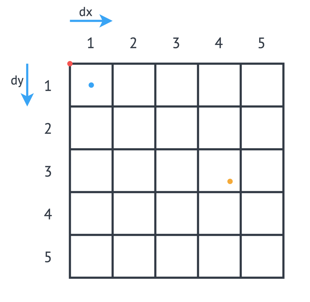
We must set the grid's origin (blue point), which represents the center of grid cell (1,1), and a size in meters for every cell in the grid. Next, we convert the cell size into a latitude and longitude distance, dy and dx respectively, and calculate the grid's top left position (red point). For any new arrival point, we can easily count how many dy and dx away the coordinates are, and therefore in the example above (yellow point), we can determine that the journey originates from cell (3,4).
The additional application logic in the Cell class and TripConvertApp performs this calculation, and we set the new record's key as the Cell type. To write to the sinkTopic, we need a new SerDes, created in an identical fashion to the one we made before.
As we chose the default partitioning strategy, records are partitioned based on the keys' different values, so this change ensures that every Trip corresponding to a particular pick-up Cell is distributed to the same partition. When we perform processing downstream, the same processing node receives all records corresponding to the same pickup cell, ensuring the operations' correctness and reproducibility.
Aggregate the data
We have now converted all of the incoming data to a type of <Cell, Trip>, and can perform an aggregation operation. Our intention is to calculate the sum of the fare_amount + tip_amount for every journey originating from one pick-up cell, across a set time period.
Because our data is historical, the time window that we use should be in relation to the original time that the events occurred, rather than the time that the event entered the Kafka system. To do this, we need to provide a method of extracting this information from each record: a class that implements TimestampExtractor. The Trip fields already contain this information for both pick-up and drop-off times, and so the implementation is straightforward—see the implementation in TripTimestampExtractor for details.
Even though the topic we read from is already partitioned by cell, there are many more cells than partitions, so each of our replicas will process the data for more than one cell. To ensure that the windowing and aggregation are performed on a cell-by-cell basis, we call the groupByKey() function first, followed by a subsequent windowing operation. As seen below, the window size is easily changeable, but for now, we opted for a window of 15 minutes.
The data can now be aggregated to generate the output metric we want. Doing this is as simple as providing an accumulator value and the operation to perform for each record. The output is of type KTable, where each key represents one particular window, and the value is the output of our aggregation operation. We use the toStream() function to convert that output back to a Kafka stream so that it can be output to the sink profit.
KStream<Cell, Trip> source = builder.stream(config.getSourceTopic(), Consumed.with(cellSerde, tripSerde));
KStream<Windowed, Double> windowed = source
        .groupByKey(Serialized.with(cellSerde, tripSerde))
        .windowedBy(TimeWindows.of(TimeUnit.MINUTES.toMillis(15)))
        .aggregate(
                () -> (double) 0,
                (key, value, profit) -> {
                    profit + value.getFareAmount() + value.getTipAmount()
                },
                Materialized.<Cell, Double, WindowStore<Bytes, byte[]>>as("profit-store")
                        .withValueSerde(Serdes.Double()))
        .toStream();
As we do not require the information of which window the values belong to, we reset the cell as the record's keys and round the value to two decimal places.
KStream<Cell, Double> rounded = windowed
                .map((window, profit) -> new KeyValue<>(window.key(), (double) Math.round(profit*100)/100));
Finally, the data can now be written to the output topic using the same method as defined before:
rounded.to(config.getSinkTopic(), Produced.with(cellSerde, Serdes.Double()));
Consume and visualize the data
We now have the windowed cell-based metric being output to the last topic, so the final step is to consume and visualize the data. For this step, we use the Vertx Kafka Client to read the data from our topic and stream it to a JavaScript dashboard using the Vertx EventBus and SockJS (WebSockets). See TripConsumerApp for the implementation.
This consumer application registers a handler that converts arriving records into a readable JSON format and publishes the output over an outbound EventBus channel. The JavaScript connects to this channel and registers a handler for all incoming messages that perform relevant actions to visualize the data:
KafkaConsumer<String, Double> consumer = KafkaConsumer.create(vertx, props, String.class, Double.class);
consumer.handler(record -> {
    JsonObject json = new JsonObject();
    json.put("key", record.key());
    json.put("value", record.value());
    vertx.eventBus().publish("dashboard", json);
});
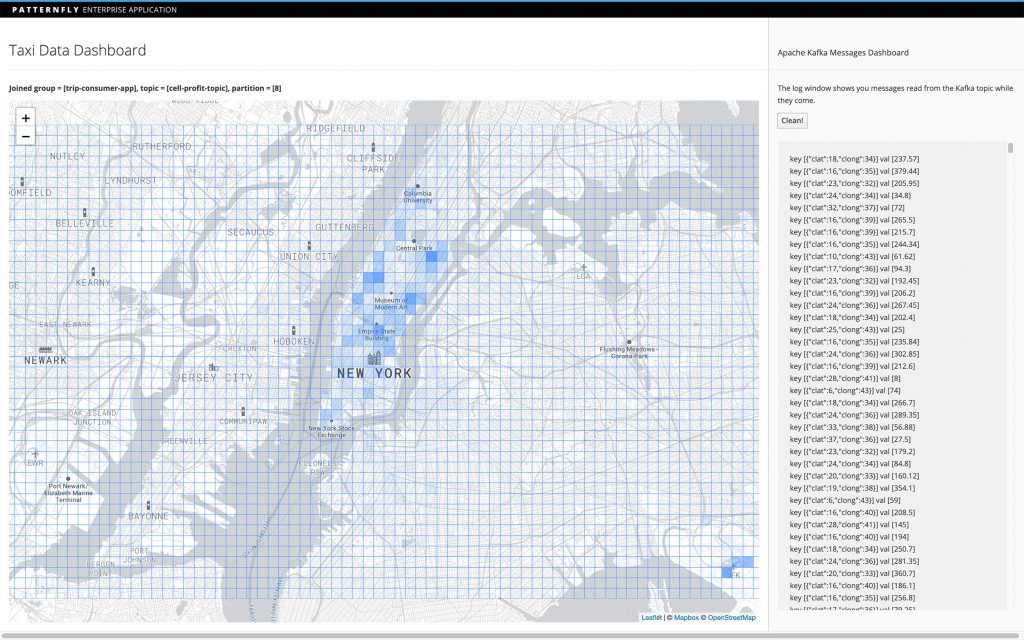
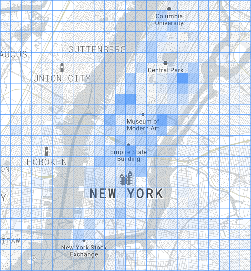
We log the raw metric information in a window so it can be seen, and use a geographical mapping library (Leaflet) to draw the original cells, modifying the opacity based on the metric's value:
By modifying the starting latitude and longitude—or the cell size—in both index.html and TripConvertApp, you can change the grid you are working with. You can also adjust the aggregate function's logic to calculate alternative metrics from the data:
Create a Kafka connector
Up until now, the producer we are using has been sufficient, even though the JAR (and image) are more bloated due to the additional data file. However, if we wanted to process the full 12GB dataset, what we have is not an ideal solution.
The example connector we built relies on hosting the file on an FTP server, but there are existing connectors for several different file stores. We picked an FTP server as it allows our connector to easily communicate with a file external to the cluster. For convenience, we use a Python library pyftpdlib to host the file with the username and password set to amqstreams. However, hosting the file on any publicly accessible FTP server is sufficient.
A Kafka connector consists of both itself and tasks (also known as workers) that perform the data retrieval through calls to the poll() function. The connector passes configuration over to the workers, and several workers can be invoked as per the tasks.max parameter. For this purpose, we created an FTPConnection class, which provides the functions we require from the Apache Commons FTPClient. On each call to poll(), we retrieve the next line from the file and publish this record to the topic provided in the configuration.
We now need to add our connector plugin to the existing amq-streams-kafka-connect Docker image, which is done by adding the JAR to the plugins folder, as described in the Red Hat AMQ Streams documentation. We can then deploy the Kafka Connect cluster using the instructions from the default KafkaConnect example, but adding the spec.image field to our kafka-connect.yamlinstead, and pointing to the image containing our plugin.
Kafka Connect is exposed as a RESTful resource, so to check which connector plugins are present, we can run the following GET request:
$ oc exec -c kafka -i my-cluster-kafka-0 -- curl -s -X GET \
    http://my-connect-cluster-connect-api:8083/connector-plugins
[{"class":"io.strimzi.TaxiSourceConnector","type":"source","version":"1.0-SNAPSHOT"},{"class":"org.apache.kafka.connect.file.FileStreamSinkConnector","type":"sink","version":"2.1.0"},{"class":"org.apache.kafka.connect.file.FileStreamSourceConnector","type":"source","version":"2.1.0"}]
Similarly, to create a new connector we can POST the JSON configuration, as shown in the example below. This new connector instance establishes an FTP connection to the server and streams the data to the taxi-source-topic. For this process to work, the following configuration options must be set correctly:
connect.ftp.address– FTP connection URL host:port.connect.ftp.filepath– Path to file on remote FTP server from root.
If needed, add this optional configuration:
connect.ftp.attempts– Maximum number of attempts to retrieve a valid FTP connection (default: 3).connect.ftp.backoff.ms– Back-off time in milliseconds between connection attempts (default: 10000ms).
$ oc exec -c kafka -i my-cluster-kafka-0 -- curl -s -X POST \
    -H "Accept:application/json" \
    -H "Content-Type:application/json" \
    http://my-connect-cluster-connect-api:8083/connectors -d @- <<'EOF'

{
    "name": "taxi-connector",
    "config": {
        "connector.class": "io.strimzi.TaxiSourceConnector",
        "connect.ftp.address": "<ip-address>",
        "connect.ftp.user": "amqstreams",
        "connect.ftp.password": "amqstreams",
        "connect.ftp.filepath": "sorteddata.csv",
        "connect.ftp.topic": "taxi-source-topic",
        "tasks.max": "1",
        "value.converter": "org.apache.kafka.connect.storage.StringConverter"
    }
}
EOF
{"name":"taxi-connector","config":{"connector.class":"io.strimzi.TaxiSourceConnector","connect.ftp.address":"<ip-address>","connect.ftp.user":"amqstreams","connect.ftp.password":"amqstreams","connect.ftp.filepath":"sorteddata.csv","connect.ftp.topic":"taxi-source-topic","tasks.max":"1","value.converter":"org.apache.kafka.connect.storage.StringConverter","name":"taxi-connector"},"tasks":[],"type":null}
We can GET the currently deployed connectors:
$ oc exec -c kafka -i my-cluster-kafka-0 -- curl -s -X GET \
    http://my-connect-cluster-connect-api:8083/connectors
["taxi-connector"]
We can check whether the data is streaming to the topic in the same way as we did in section Send data into Apache Kafka. For debugging information, see the logs for my-connect-cluster-connect. To stop the plugin, we can delete it with the following command:
$ oc exec -c kafka -i my-cluster-kafka-0 -- curl -s -X DELETE \
    http://my-connect-cluster-connect-api:8083/connectors/taxi-connector
That's it. We managed to create a more complex Red Hat AMQ Streams application where we source historical real-world data with a Kafka Connector, stream it through multiple processing points, and sink it to a visualization.
Read more
Building Apache Kafka Streams applications using Red Hat AMQ Streams: Part 1
Last updated: March 28, 2023