In How to build an AI-driven product recommender with Red Hat OpenShift AI, we explored how Red Hat OpenShift AI supports the underlying technologies used by the product recommender. This post examines the architecture and training behind the recommender's two-tower model. First, let's get our bearings and review the strategy our two-tower training pipeline implements.
Training the two-tower model
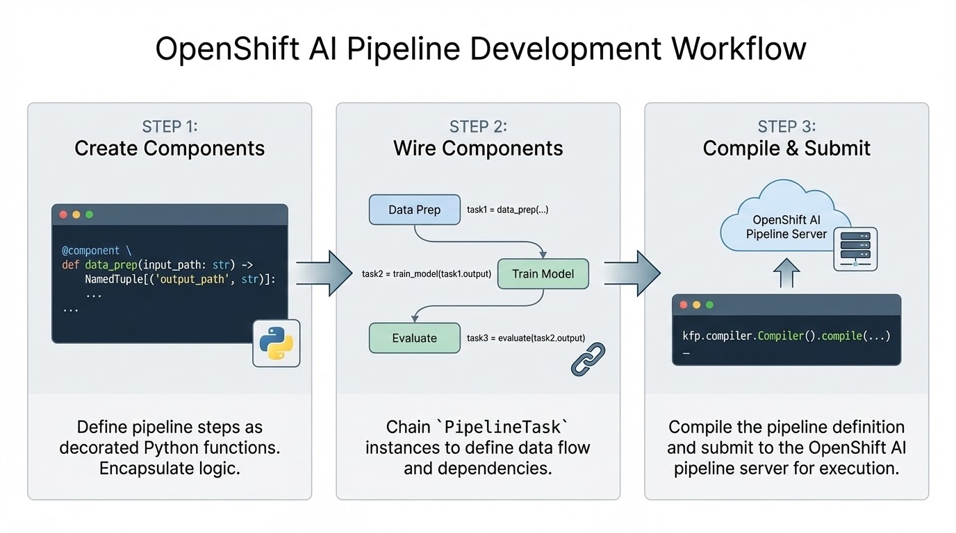
OpenShift AI integrates with KFP and workflow managers like Argo Workflows and Tekton. This allows engineers to design their training pipelines into functional components like those shown in Table 1. OpenShift AI simplifies lower-level details like containerization, deployment, data sharing between pipeline stages, retries, and monitoring.
A regular Python function decorated with the @kfp.dsl.component tag represents each task in Table 1. The component tag specifies the system and library dependencies the code requires; the function's parameter signature defines the data it consumes and generates.
| Task/Stage | Description |
|---|---|
| Load training data | Loads historic and new user, product and user-product interaction data (for example, purchases, cart additions). |
| Train model | Pre-processes data and computes user-product interaction magnitudes (explained in detail later). Trains two-tower model to create user and product encoders in a shared embedding space. |
| Generate candidates | For each user embedding, determines top similar product embeddings and pushes results to Feast as a quick recommendations lookup table for each user ID. |
The batch_recommendation function, which is decorated with the @kfp.dsl.pipeline tag, wires the overall pipeline together:
@dsl.pipeline(name=os.path.basename(__file__).replace(".py", ""))
def batch_recommendation():
    load_data_task = load_data_from_feast()
    train_model_task = train_model(
        item_df_input=load_data_task.outputs["item_df_output"],
        user_df_input=load_data_task.outputs["user_df_output"],
        interaction_df_input=load_data_task.outputs["interaction_df_output"],
    ).after(load_data_task)
Engineers set the pipeline's execution order in this function by chaining components together with the after() method. Though the preceding code shows the component functions being invoked, the KFP DSL is a Python decorator that wraps the original function to defer its execution and instead return a PipelineTask instance that supports the methods shown in the code example.
These methods help engineers connect tasks, specify task resource details, and access task output data during execution. The pipeline server executes the core training stages listed in Table 1 once the pipeline is compiled and submitted to the pipeline server:
pipeline_yaml = "train-workflow.yaml"
compiler.Compiler().compile(pipeline_func=batch_recommendation, package_path=pipeline_yaml)
# The endpoint for the pipeline service
client = Client(host=os.environ["DS_PIPELINE_URL"], verify_ssl=False)
pipeline_name = os.environ["PIPELINE_NAME"]
uploaded_pipeline = client.upload_pipeline(
    pipeline_package_path=pipeline_yaml, pipeline_name=pipeline_name
)
run = client.create_run_from_pipeline_package(
    pipeline_file=pipeline_yaml, arguments={}, run_name=os.environ["RUN_NAME"]
)
logger.info(f"Pipeline submitted! Run ID: {run.run_id}")
When the pipeline is configured and submitted to the pipeline server, OpenShift integrates a configured workflow engine (like Argo Workflows or Tekton) to containerize and deploy each component in a dedicated pod. Tasks can share data with one another using either scalar parameters or KFP artifacts (these are typically machine learning datasets).
For example, the load_data_from_feast component generates three datasets that hold product, user and user-product interactions. The train_model component indicates its dependency on this data and its parameter signature:
@dsl.component(base_image=BASE_IMAGE,
               packages_to_install=["minio", "psycopg2-binary"])
def train_model(
    item_df_input: Input[Dataset],
    user_df_input: Input[Dataset],
    interaction_df_input: Input[Dataset],
    item_output_model: Output[Model],
    user_output_model: Output[Model],
    models_definition_output: Output[Artifact],
):
Figure 1 summarizes the overall development workflow.
OpenShift AI's integration with KFP and Argo Workflows provides several benefits, including simplifying task-specific library dependencies (each function can specify its own versioned library dependencies without requiring developers to maintain multiple container images manually), failure recovery and a simplified parallel execution abstraction. PipelineTask instances that are not explicitly chained together and that do not have implicit input/output dependencies can be executed in parallel to better utilize the cluster's resources.
While the abstractions provided by OpenShift AI and KFP are convenient, data engineers must consider multiple factors in their pipeline design in order to achieve an optimal level of parallelization and performance. Greater parallelization is achieved by decomposing the pipeline into independent components.
For example, the load_data_from_feast component currently loads and pre-processes three separate datasets. While a single function can improve code readability and maintainability, KFP would be able to prepare the three datasets in parallel if the engineer decomposes this step into an independent component for each dataset.
Another design aspect which data engineers must consider is how the components share data with one another, which we discuss next.
How KFP enables data sharing
We mentioned earlier that the train_model component can access data produced by the load_data_from_feast stage. The load_data_from_feast function simply writes the data it's prepared to its local file system using the parquet format. The train_model function, which is the subsequent pipeline task, reads this same parquet data from its local ephemeral file system.
But how can this work? In OpenShift (and Kubernetes in general), pods are not permitted access to each other's local ephemeral storage (even when they are scheduled on the same node).
KFP bridges normal pod isolation using a kfp-launcher init container to prepare each pod's local ephemeral storage with the data it needs based on the information engineers provide in the KFP decorators we discussed earlier. Data is copied between pods using the pipeline's configured S3-compatible storage (MinIO in our case), effectively allowing engineers to treat cloud object storage as local file storage. S3-compatible storage also ensures the data lineage and logs for each pipeline run are preserved after the run has completed and all its ephemeral pods have been terminated.
Alternatives to the input/output pattern
While the usage pattern described above provides a convenient abstraction, it is not suitable for machine learning jobs with large datasets that exceed the pod's limited local ephemeral storage, especially on busy clusters where multiple pods must contend for storage on the same node. If a pod reaches its configured upper limit on storage use or its node nears its maximum, the node's eviction manager might abruptly terminate the pod to avoid out-of-disk-space errors on the node.
Fortunately, there are several supported alternatives to direct artifact sharing in KFP, such as techniques that only share the location of shared data between pods (versus a full copy). Another option is to use Feast or another external data storage solution as a shared storage pool across pods. Keep in mind, however, that externally managed storage solutions will impact the observability of each run's data lineage in the OpenShift AI dashboard.
KFP pod allocation
Before we leave the topic of ML pipelines, it's useful to note that the code that submits a compiled pipeline to the cluster will result in multiple ephemeral pods. This can be confusing to data engineers when they are troubleshooting. Table 2 lists these pods and their function (the id portion of pod names is replaced with random strings during execution).
| Pod name | Function | Count |
kfp-run-job | Runs the __main__ code in our train-workflow.py, which compiles and submits the pipeline to the pipeline service in OpenShift. | 1 |
train-workflow-id-system-dag-driver | Responsible for coordinating all tasks in their proper execution order | 1 |
train-workflow-id-system-container-driver | These pods are created for each pipeline task and provide several critical functions including the creation and submission of a pod specification for each task, pod monitoring and retry logic implementation and management of each task's output data. | 3 (1 per task) |
train-workflow-id-system-container-impl | This is where the developer's task-specific code executes. | 3 (1 per task) |
Two-tower (dual encoder) architecture
Now that we've covered how OpenShift AI's integrated pipeline server helps engineers create ML models, let's turn to the specifics of how the two-tower model creates a shared embedding space for products and users.
Overview
The dual encoder trains two neural networks–one for user features and one for product features–on a common objective. Here, our objective is to align the proximity of the embeddings with a score that reflects how well the two entities were paired historically. The function returns larger values for interactions that were negative (for example, if the user gave the product a bad rating) and smaller values for positive interactions (for example, if the user purchased the product).
The function works as a loss function for backpropagation because the score is the inverse of the user's sentiment. Specifically, for each batch of historic user-product interactions, the mean squared error (MSE) is computed for the distance between the embeddings and their scalar magnitude scores. Backpropagation updates each network's weights to reduce this error. After the error converges, the two networks can generate user and product vectors in the same embedding space.
Detailed architecture
The user and product embedding networks are each an instance of the architecture shown in Figure 2. You can find the code for this network in entity_tower.py under the recommendation_core project as the EntityTower Python class.
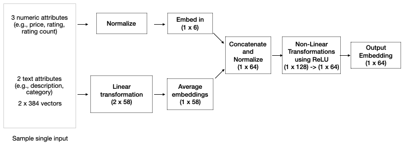
Each instance of the EntityTower is a simple feedforward network that processes multiple numeric and text features for an input entity (for example, a user or product) to produce a 64-component embedding. A prior step in the training pipeline converts text inputs to 384-component embeddings using the BGE model (See LLMs and machine learning models). The EntityTower linearly transforms each 384-component embedding per text attribute (for example, product name, description) to separate 58-component embeddings and averages them.
The numeric features are normalized to account for potentially different scales and levels of variance (for example, product price versus rating), and the results are linearly transformed to a 6-unit layer. The two layers are concatenated and normalized to a single 64-unit layer and processed through two non-linear transformations that first expand the output to 128 components, then back to 64. Normalization at the input and intermediate layers provides several benefits, including reduced training time and improved model accuracy.
By itself, the EntityTower is only a feed-forward network. It applies matrix computations to the inputs, but it cannot learn anything without an objective, such as a loss function to minimize.
This is precisely why the two-tower architecture shown in Figure 3 is needed. The EntityTower is instantiated twice to separately process user and product attributes. The two-tower network computes the Euclidean distance between the embeddings produced by the two EntityTower instances and compares these distances to the magnitude scores for the user-product interaction.
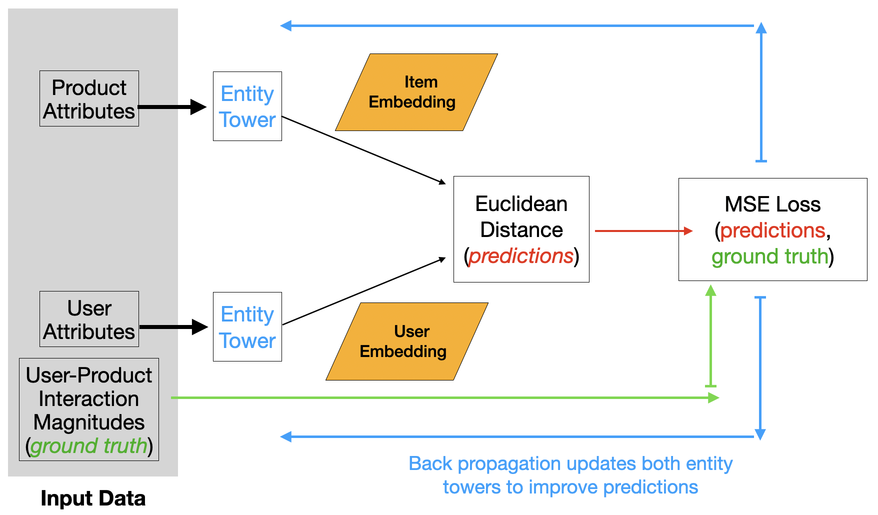
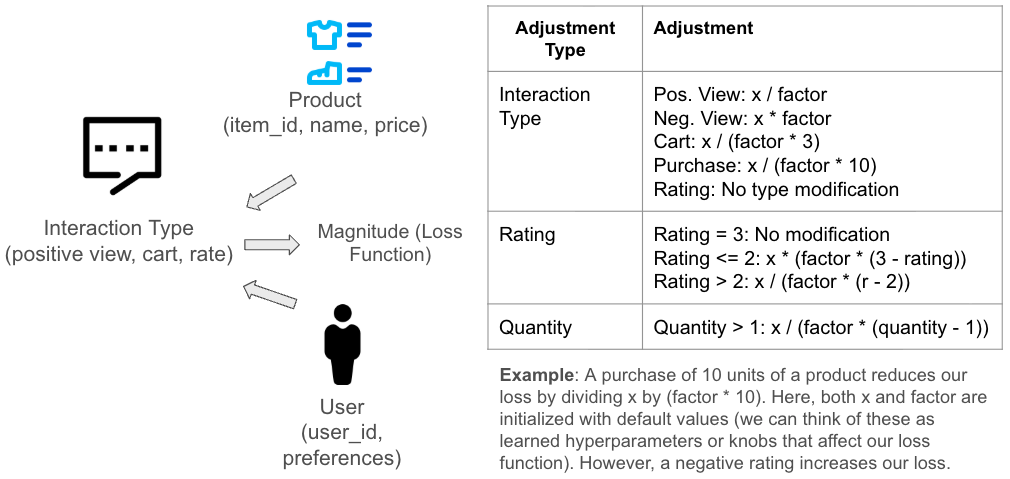
Figure 4 depicts the details of this magnitude scoring function for each interaction type (for example, purchases, ratings, cart additions). Note, for example, how the function magnifies the impact of some interaction types like purchases using additional data, like the number of products purchased.
Once the two-tower network is trained, we can compute the embeddings for any user using the EntityTower for the user's attributes (the user encoder) and then search for nearby product embeddings created by the EntityTower for the product attributes (the product encoder) to generate a list of recommended products.
Recommendations for newly registered users
The AI quickstart employs a scheduled job that runs nightly to pre-compute recommendations and store them in Feast for fast retrieval later when users log in. Because newly registered users will not have an entry in this fast lookup table, the AI quickstart employs a different recommendation technique until the next scheduled recommendation job executes.
The registration process prompts the user for product categories to gauge their preferences. The application uses the category preferences to show related products. Selected products are saved as positive interactions for future two-tower training. In the meantime, the user's selected categories are used as general preferences to make recommendations. Specifically, the AI quickstart returns the most popular products in those categories.
This approach addresses the classic “cold start” problem without using expensive operations. Alternatively, you can use the user encoder to create an embedding and compare it against a list of precomputed embeddings created by the product encoder. Even if the user encoder lacks specific information about a new user, it uses patterns from other users and products to produce quality recommendations.
Limitations of recommender model
It's important to note that the model's architecture and dataset are notional and meant as a simple example to demonstrate OpenShift AI's capabilities. A more realistic recommender model would consider additional factors like the following:
- Additional normalization layers applied to every activation layer in the network.
- An appropriate split between numeric and text weights for a domain's features. In our case, the split favors text data (58 versus 6 output units just before the concatenation layer in Figure 2). This would not be appropriate for a financial application, for example, which has hundreds of numeric features and only a few text features.
- Alternative transformation layers. For example, instead of a simple expansion block at the end of the network, consider a more traditional bottleneck layer that compresses the learned weights. Autoencoders apply this architecture as a regularization technique to force the model to learn the most important patterns in the input.
- Most recommenders in production also consider numerous user and product features, such as age and demographics.
- While the MSE loss function is easy to understand, consider multiple architectural modifications to support alternatives like Cross-Entropy loss.
OpenShift AI's workbenches with pre-loaded images that support PyTorch are an excellent way to experiment with these different training approaches and evaluate their performance. The best approach for your specific data will often reveal itself only through experimentation.
In the final installment of this article, we discuss how the product recommender uses generative AI to summarize product reviews. Read it here: AI-generated product review summaries with OpenShift AI
Explore more use cases in the AI quickstart catalog.
Last updated: February 2, 2026