Visualize Performance Co-Pilot data with geomaps in Grafana

In this blog post, I explain the geomap visualization in Grafana and how it can be used with Performance Co-Pilot (PCP) and grafana-pcp, a Grafana app plug-in for PCP, to visualize performance data from systems you want to monitor.

Grafana geomaps enable viewing data in a world map, in addition to altering the map based on that data. This is highly useful when observing data coming from different locations that has coordinate data associated with it.

PCP is a performance monitoring tool that can be configured to monitor many systems across different locations. In PCP, metric values have labels associated with them that include additional metadata (for example, a hostname). Historically, the labels didn't include coordinate data. The addition of the pcp-geolocate package now enables adding longitude and latitude labels to metric values. For more information, read the PCP documentation.

The grafana-pcp plug-in enables visualizing PCP data with coordinate labels in a Grafana geomap panel. This functionality is available in Red Hat Enterprise Linux 10.1 (RHEL) and comes with many use cases, like getting a quick overview of all your systems. The geomap panel provides plenty of options to cater to many requirements. Read the Grafana documentation for more information on the grafana-pcp plug-in.

System setup

First, you must install PCP, Grafana, and grafana-pcp on your system. You must also install the pcp-geolocate package that handles attaching coordinate labels (longitude and latitude) to your metrics. Here are the commands to properly set up your system:

dnf install pcp-zeroconf valkey grafana-pcp pcp-geolocate
systemctl restart valkey pmproxy grafana-server pcp-geolocate
systemctl enable valkey pmproxy grafana-server pcp-geolocate

To verify that the longitude and latitude labels are present in your Valkey database, use the pmseries command-line tool to list the labels associated with metric values:

pmseries --labels

This command shows you all the PCP labels on your system, including the longitude and latitude labels.

You can also check a PCP archive file for the longitude and latitude labels:

pminfo --labels --archive <archive_file> <metric>

The PCP Valkey datasource is the only grafana-pcp datasource that has support for geomaps. Read the grafana-pcp quickstart guide for instructions on setting up the grafana-pcp plug-in and the datasources, including PCP Valkey.

Creating a geomap for the PCP Valkey datasource from grafana-pcp

To create the geomap, open Grafana and navigate to Dashboards and create a new dashboard. When prompted to select a datasource, pick the PCP Valkey datasource you have configured.

Next, change the visualization to a geomap. Open the Format drop-down menu located at the bottom of the query window and select Geomap.

Enter your query (the PCP metric of interest) in the query window to see your PCP data visualized on the map. Figure 1 shows a geomap dashboard visualizing the kernel.all.pswitch metric from 2 different systems on opposite sides of the world.

Getting your data visualized on a world map can be immediately helpful, but a lot of the power of the geomap is in the options and configurations. In Figure 2, the location with the higher value is red, while the location with the lower value is green. This was made possible by setting a threshold.

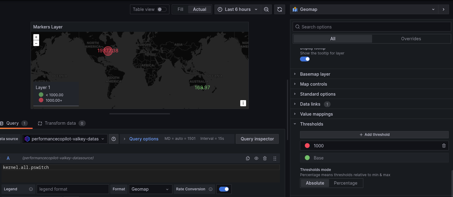
In the editing window for the panel, the threshold is set to 1,000 and the color red, so any location with a value above 1,000 appears as a red marker on the map. This can be helpful in finding a system that is not performing within acceptable performance limits and needs to be checked for a potential problem.

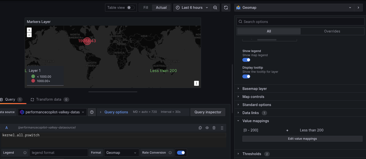
Value mappings are another useful geomap option. With this option, you can map certain values to a message. For example, you could map values in the range of 0-200 to the message "Less than 200" to see a text message on the geomap (Figure 3). This is useful for showing the locations within acceptable performance limits without worrying about what that actual value is.

More geomap options and next steps

This article has demonstrated only a small subset of what can be done with geomaps. There are other layers too, like heatmap layers that can be used rather than the markers layer used in the example. The full geomap documentation explains the different layers and options available in Grafana.

I recommend experimenting with different layers and options to see what works best for you. Geomaps excel at providing a quick and visually appealing overview of all your locations in a single panel. Finding which options help you easily find locations in need of further investigation unlocks the power of the geomap.