Page
Prerequisites and step-by-step guide
Prerequisites:
- Introduction to OpenShift AI
- Red Hat Developer Sandbox
- GitHub
- Prior knowledge of Python
Step-by-step guide:
Step 1: Launch JupyterLab
- Navigating to the OpenShift AI Dashboard:
Choose Red Hat OpenShift AI in the bottom right area of the "Available services" section. You can click on "Launch", as shown in Figure 1 below.
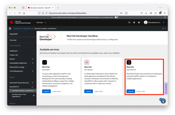
Figure 1: The Red Hat Hybrid Cloud Console with Red Hat OpenShift AI. 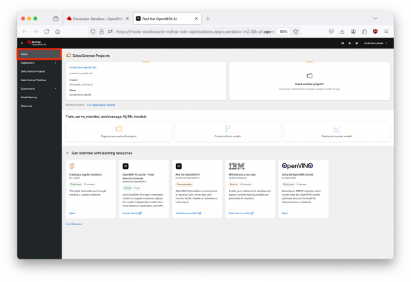
Figure 2: Red Hat OpenShift AI Dashboard. Once you have completed the previous step of selecting the OpenShift AI Sandbox, it would take you to the Red Hat Open Shift AI dashboard. The interface includes a navigation menu on the left with options like "Home," "Applications," "Data Science Projects," "Data Science Pipelines," "Experiments," "Model Serving," and "Resources". Navigate to the "Home" as shown in Figure 2 above.
- Selecting Your Data Science Project:
- Creating a New Workbench:
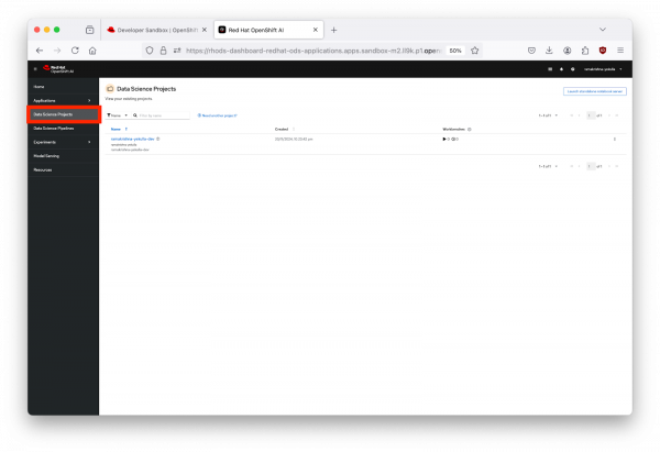
- Click on your project name from Figure 3, and then navigate to the "Workbenches" section in the main content area as highlighted in Figure 4 below.
- Initiate a New Workbench:
Click on "Create a Workbench".
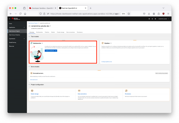
Figure 4: Create Workbench Interface. - Configuration, as shown in Figure 5 below:
- Name: Give it a descriptive name, e.g., "interactive_classification".
- Notebook Image: Select TensorFlow, as our model will use this framework.
- Deployment Size: Choose "Medium" for a balanced performance.
- Cluster Storage: Allocate 20 GiB to ensure you have enough space for datasets and models.
Launch the workbench by clicking "Create Workbench" and wait for the status to indicate its "Running", as shown in Figure 6.
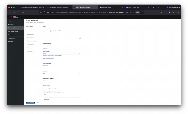
Figure 5: Configuration of a New Workbench. 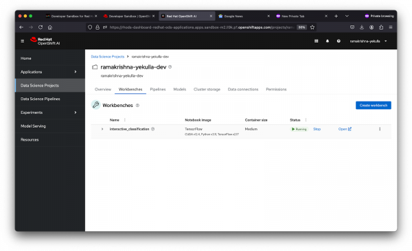
Figure 6: Running Workbench.
Step 2: Obtain and Prepare the Dataset
Purpose:
- To automate the fetching of datasets using Kaggle's API, simplifying data preparation in AI projects.
Why:
- Using the Kaggle API key enables direct access to large datasets for machine learning, enhancing data acquisition efficiency.
Download Your Kaggle API Key
- Access Your Kaggle Account:
- Navigate to the Kaggle website and log in with your account credentials.
- Go to Account Settings:
- Click on your profile icon at the top right corner of the page, then select Account from the dropdown menu as shown below in Figure 7.
- Download API Key:
- Scroll down to the section labeled API. Here, you'll find a Create New Token button. Click this button.
A file named kaggle.json will be automatically downloaded to your local machine. This file contains your API credentials. Check in your Downloads directory for the kaggle.json
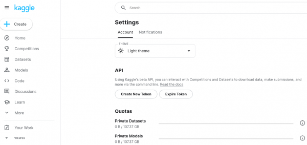
Figure 7: Kaggle API Download. 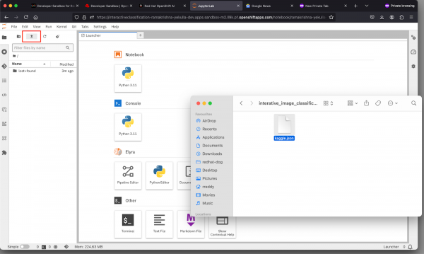
Figure 8: Kaggle API Setup in JupyterLab.
Setup the API Key on your Workbench:
- Access your JupyterLab IDE environment:
- Log into the OpenShift AI dashboard and navigate to your JupyterLab instance.
- Upload the API Key:
- If you have successfully completed the Download API Key from kaggle portal, A file named kaggle.json will be automatically downloaded to your local machine.
- If you haven't already, upload the kaggle.json file to your JupyterLab IDE environment. You can drag and drop the file into the file browser of JupyterLab IDE as shown in Figure 8 above. This step might visually look different depending on your Operating System and Desktop User interface.
- Clone the Interactive Image Classification Project:
- At the top of the JupyterLab interface, click on the "Git Clone" icon.
- Enter the GitHub URL: in the popup window.https://github.com/redhat-developer-demos/openshift-ai.git
- Click the "Clone" button.
- After cloning, navigate to the openshift-ai/2_interactive_classification directory within the cloned repository.
Open the Python Notebook in the JupyterLab Interface
- The JupyterLab interface is presented after uploading kaggle.json and cloning the openshift-ai repository – showing the file browser on the left with 'openshift-ai' and '.kaggle.json' as shown in Figure 9 below. Open Interactive_Image_Classification_Notebook.ipynb in the openshift-ai directory and run the notebook, The notebook contains all necessary instructions and is self-documented.
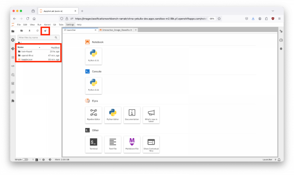
Figure 9: Post-Clone Repository View in JupyterLab. Execute the Cells in the Python Notebook
- Start by executing each cell in order by pressing the play button or using the keyboard shortcut "Shift + Enter" as shown in Figure 10 below.
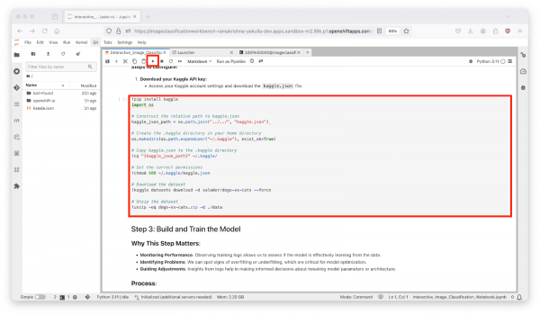
Figure 10: Running the Interactive Classification Notebook.
Step 3: Build and Train the Model
- Data Preparation: Set up data generators for preprocessing images through scaling, augmentation, or normalization to enhance training efficiency. Architect the CNN with convolutional, pooling, and dense layers to extract and classify image features.
- Model Training:
- Compile: Use an optimizer, loss function, and metrics like accuracy.
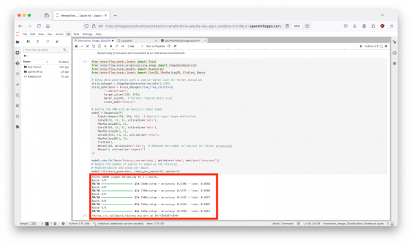
- Train: Model adjusts weights through backpropagation to reduce loss over 5 epochs, with each epoch broken into 50 steps. In the Output: "Found 20000 images belonging to 2 classes." This dataset has 20,000 images divided into 'cats' and 'dogs', ensuring a balanced dataset for equitable model learning. This ensures you have enough data to train on, and that the classes are balanced, which is crucial for model fairness.
This step-by-step analysis equips learners with the tools to interpret training outputs, troubleshoot issues like overfitting or underfitting, and refine their models to achieve better performance. This summary and analysis from training logs are essential for learners to understand model performance dynamics, diagnose issues, and strategize improvements in machine learning projects. In the output as shown in Figure 11 below, you can see the CNN model training process with code cells and output logs. The output section at the bottom displays the training progress with accuracy and loss metrics for each epoch, including final accuracy: 0.5359 and final loss: 0.6915.
Step 4: Interactive Real-Time Data Streaming and Visualization
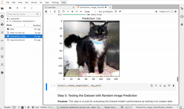
We simulate real-time data interaction and demonstrate how AI can be used interactively in a simplified context. We leverage TensorFlow and ipywidgets to simulate real-time data streaming and visualization.
Process:
- Create Interactive Dropdown Menus: Implement dropdown menus to allow users to select and visually interact with predictions on cat or dog images.
- Utilize Widgets for Simulation: Use Jupyter Notebook widgets to simulate real-time data streaming. This approach is particularly useful for educational and demonstration purposes, showing how data can be dynamically processed and visualized in an interactive environment.
Once you run the cell in Step 4 , you should see an output as shown in Figure 12 below.
Step 5: Testing the Dataset with Random Image Prediction
This step is crucial for evaluating the trained model's performance by testing it on unseen data in a real-world-like scenario. By randomly selecting images and predicting their classes, we can visually assess the model's accuracy and reliability. Run the cell in Step 5 as shown in Figure 13 below.
Process:
- Random Image Selection: The function predict_random_image takes a directory path as input and checks if the path exists. It then randomly selects an image from this directory, ensuring that each test is unbiased and represents a realistic use case.
- Image Loading and Preprocessing: The randomly chosen image file is then loaded and preprocessed to match the input format expected by the model. This involves resizing the image and normalizing its pixel values.
- Model Prediction: The preprocessed image tensor is fed into the model to predict whether the image is of a 'Cat' or a 'Dog'. This step directly utilizes the neural network to interpret the image data.
- Visualization: The image along with its predicted class is displayed. This visual feedback is crucial for understanding the model's decision-making process and immediately seeing the result of the prediction.
Interactive Testing: By running the function with different directories (e.g., cats and dogs), users can interactively test how the model performs across varied inputs, making this a dynamic tool for demonstration and educational purposes. Testing the model with a random selection of images simulates how the model might perform in a production environment where inputs are not predetermined. It helps in identifying potential biases, underfitting, or overfitting issues in the model. Additionally, visual feedback from test predictions is an excellent way to demonstrate the model's capabilities to a non-technical audience, making complex machine learning concepts more accessible and understandable.
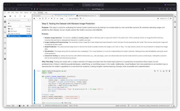
Figure 13: Testing the Dataset with Random Image Prediction. You should now see an output of two images, one of a cat and one of a dog, with their respective predictions labeled as "Cat" and "Dog". as shown in Figure 14 below.
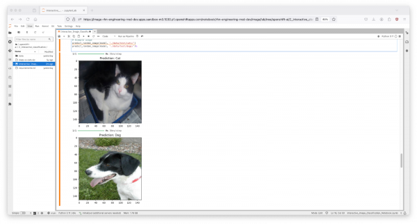
Figure 14: Image Classification Predictions in Jupyter Notebook.
Step 6: Interactive Real-Time Image Prediction with Widgets
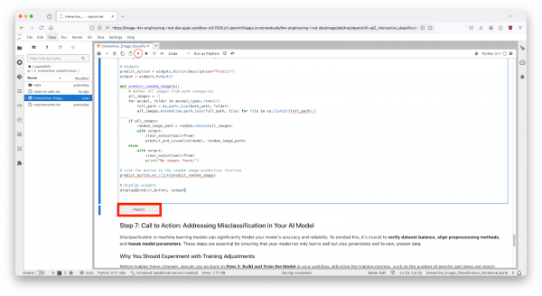
Purpose: This step integrates interactive web widgets to provide a user-friendly interface for real-time image prediction, showcasing how TensorFlow and Jupyter Notebook widgets can be used to enhance the interactivity and accessibility of AI applications.
Output:
- Once the code in the cell is executed in Step 6, a predict button would appear as shown in Figure 15 above. The interactive session will display images with their predicted labels in real-time as the user clicks the "Predict" button. This dynamic interaction helps in understanding how well the model performs across a random set of images and provides insights into potential improvements for model training.
Step 7: Addressing Misclassification in Your AI Model
Misclassification in machine learning models can significantly hinder your model's accuracy and reliability. To combat this, it's crucial to verify dataset balance, align preprocessing methods, and tweak model parameters. These steps are essential for ensuring that your model not only learns well, but also generalizes well, to new, unseen data.
Why You Should Experiment with Training Adjustments
Before making these changes, ensure you go back to Step 3: Build and Train the Model in your workflow. Adjusting the training process, such as the number of epochs and steps per epoch, can provide quicker feedback on model performance, allowing you to iteratively improve your model in a more controlled and informed manner. Here’s what you can do:
Adjust the Number of Epochs to Optimize Training Speed
Changing the number of epochs can help you find the sweet spot where your model learns enough to perform well without overfitting. This is crucial for building a robust model that performs consistently.
Try Different Values for Steps per Epoch
Modifying steps_per_epoch affects how many batches of samples are used in one epoch. This can influence the granularity of the model updates and can help in dealing with imbalanced datasets or overfitting.
Example Code to Modify Your Training Process
Make these modifications in your Notebook or another Python environment as part of "Step 3: Build and Train the Model". Here’s how you might modify the training to see how these changes can impact your model's learning curve and overall performance:
# Adjust the number of epochs and steps per epoch
model.fit(train_generator, steps_per_epoch=100, epochs=10)Summary
By following this tutorial, you not only gain practical experience in image classification but also develop the skills necessary to extend these methods to more complex and diverse datasets. Whether for educational purposes or professional projects, the knowledge you acquire here sets a solid foundation for future exploration and innovation in the field of artificial intelligence.
