As Red Hat OpenShift finds its way into more on-premise data centers, we're seeing more network interface card (NIC) bonding for that sweet spot of high availability and performance. Before you jump in, there are a few things to mull over when picking your NIC bond configuration. So, let's dive into these considerations and see what the performance numbers tell us.
Quick hits: What you need to know
There are key things to keep in mind regarding NIC bond configuration:
- Only layer2/layer2+3 transmit policies are actually 802.3ad compliant.
- You might see out-of-order packet delivery if you go with non-compliant transmit modes like layer3+4 or encap3+4.
- The way Red Hat OpenShift Container Platform hands out MAC addresses can sometimes cause the hashing algorithm to favor one interface when you're bonding two. This is a known issue tracked at Red Hat.
- Ultimately, the best bonding mode really hinges on how your application’s architecture and how it uses the network.
Why should you care about xmit-hash?
Choosing the right transmit hash algorithm isn't just a "set it and forget it" kind of deal. It's important to think about the kinds of applications you'll be running on OpenShift. Are you going to have numerous pods chattering away on each node, or just a few pods (or maybe even one) making point-to-point connections?
- If your setup involves many pods needing network access, layer2/layer2+3 could be your best bet because it helps spread traffic across those bonded links.
- On the flip side, if your application doesn't create a swarm of pods (i.e., one pod per node), layer3+4 might be the preferred choice. This is especially true if your app is good at using different source ports or destination points for each network stream it creates.
What we're working with: The test setup
To get to the bottom of this, we put together a specific test environment. Figure 1 shows a quick sketch of what our system under test (SUT) looks like.

Our lab features a single Juniper QFX5200 as our Top of Rack (ToR) switch. There are no fancy dual switches for redundancy in our setup. But don't worry, the test results wouldn't change if you properly configure the switch infrastructure.
The gear
All our machines are identical to keep things consistent:
- Servers: Dell R660 with Intel(R) Xeon(R) Gold 5420+ CPUs and a hefty 512Gi of RAM.
- Bonded NIC: Mellanox Technologies MT2892 Family (ConnectX-6 Dx) on the R660, with a speed of 200000Mb/s.
- NIC details: Each NIC port is 100000Mb/s, using the mlx5_core driver and firmware version 22.36.1010.
The software stack
Just like the hardware, the software is the same across the board:
- OpenShift: Version 4.18 (though we also ran tests on older versions like 4.14).
- Kernel: 5.14.0-427.66.1.el9_4.x86_64.
Our testing tool: k8s-netperf
For our tests, we relied on an upstream tool called k8s-netperf. It's built by Red Hat Performance engineers specifically to measure network performance in Kubernetes setups. In this article, we're zeroing in on a simple TCP Stream between a single client and server pod, each running on different OpenShift worker nodes.
Here's a peek at our k8s-netperf configuration (netperf.yml):
---
tests:
  - TCPStream:
    parallelism: 1
    profile: "TCP_STREAM"
    duration: 30
    samples: 5
    messagesize: 4096
  - TCPStream:
    parallelism: 2
    profile: "TCP_STREAM"
    duration: 30
    samples: 5
    messagesize: 4096
  # ... (and so on for 4, 8, 16, 20 parallel streams)
This is how we kicked off the tests:
$ k8s-netperf --metrics --iperf --netperf=false --clean=false --all --debugHeads up:
This article won't walk you through setting up OpenShift with bonds. We're assuming you've already got that up and running in your lab.
Hashing: Layer2 (the default)
If you just go with the standard Link Aggregation Control Protocol (LACP) bond configuration, your transmit (xmit) policy will be set to layer2(0). This method looks at the source (src) and destination (dst) MAC addresses to make its hashing decisions. In our OpenShift world, OVNKubernetes actually generates these MAC addresses from the IP addresses.
The kernel documentation tells us it uses an XOR of the hardware MAC addresses and the packet type ID to create the hash. The basic formula is as follows:
Uses XOR of hardware MAC addresses and packet type ID
field to generate the hash. The formula is
hash = source MAC XOR destination MAC XOR packet type ID
slave number = hash modulo slave count
This algorithm will place all traffic to a particular
network peer on the same slave.
This algorithm is 802.3ad compliant.
This approach keeps all traffic to a specific network peer on the same slave interface and is 802.3ad compliant.
Figure 2 shows the packet flow.
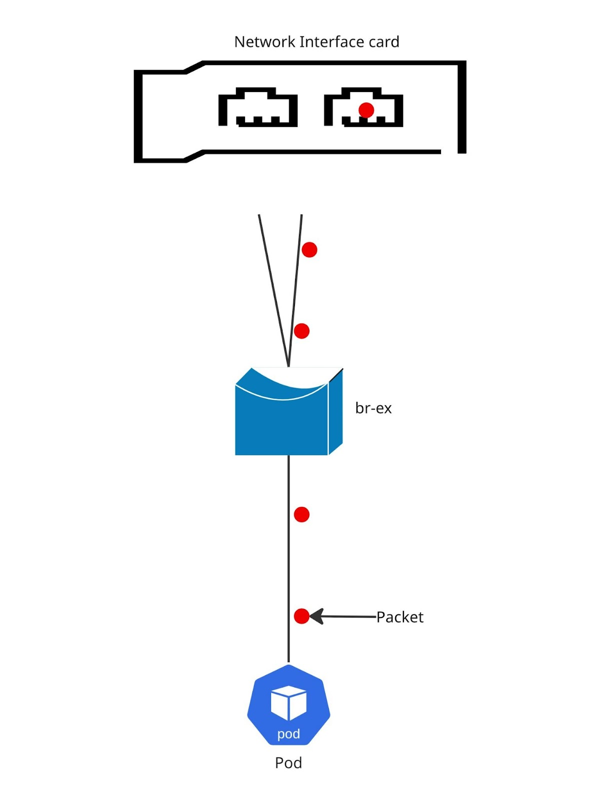
Layer2 results
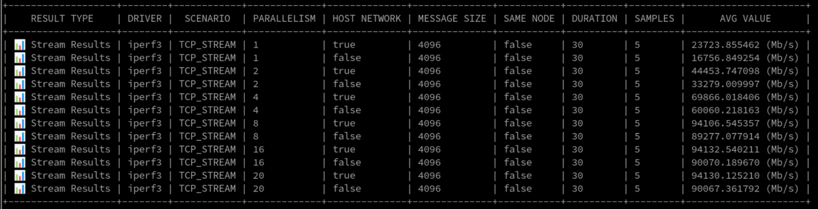
With a single stream within the pod network, we clocked speeds of over 16 Gbps. When running on the host network, this jumped to more than 23 Gbps. When we cranked it up to 8 iPerf3 streams, we saw throughput max out around a whopping 90Gbps.
Check out the network utilization during this test in Figure 3. You can see one interface doing most of the heavy lifting for transmission, which is expected with this hashing mode and a single destination.

For the data lovers, here's a snippet of the raw results (Figure 4).
Layer2+3 hashing
Moving on to Layer2+3 hashing, the algorithm is similar to Layer2 but throws IP addresses into the mix. Interestingly, our tests highlighted an area for improvement in how OVNKubernetes creates MAC addresses for pods. Currently, OVNKubernetes derives the MAC address from the IP address assignment. This predictability doesn't play super well with hashing when you're just using two interfaces in your bond. We've actually put in a Request For Enhancement (RFE) to make MAC assignments random instead of predictable. (Remember, Linux hashes the last byte of the MAC here too.)
From the kernel docs, this policy uses a combo of layer2 and layer3 info. The formula expands to:
This policy uses a combination of layer2 and layer3
protocol information to generate the hash.
Uses XOR of hardware MAC addresses and IP addresses to
generate the hash.  The formula is
hash = source MAC XOR destination MAC XOR packet type ID
hash = hash XOR source IP XOR destination IP
hash = hash XOR (hash RSHIFT 16)
hash = hash XOR (hash RSHIFT 8)
And then hash is reduced modulo slave count.
If the protocol is IPv6 then the source and destination
addresses are first hashed using ipv6_addr_hash.
This algorithm will place all traffic to a particular
network peer on the same slave.  For non-IP traffic,
the formula is the same as for the layer2 transmit
hash policy.
This policy is intended to provide a more balanced
distribution of traffic than layer2 alone, especially
in environments where a layer3 gateway device is
required to reach most destinations.
This algorithm is 802.3ad compliant.
The packet flow looks quite similar to Layer2. If we had more pods acting as clients and servers, we'd likely see better traffic balancing across the bond. This should get even better once the OCPBUGS-56076 issue (the RFE about random MACs) is addressed.
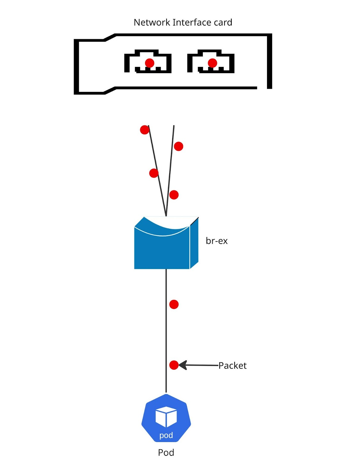
Figure 5 shows the packet flow for Layer2+3.
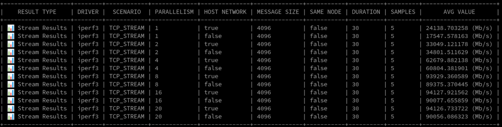
Layer2+3 results
Because Layer2+3 is so close to Layer2, and we were testing with a single source and destination, the hash algorithm pretty much stuck to a single interface in the bond. As expected, the performance wasn't drastically different from what we saw with Layer2.
The utilization graph in Figure 6 tells a similar story, with one interface handling the bulk of the transmission.

Figure 7 shows the raw numbers.
Layer3+4 hashing
Now for Layer3+4 hashing. This approach can give you the highest throughput for multiple streams of communication, even from a single source to a single destination. Layer3+4 considers the IP address, source port, and destination port. So, if your application is savvy enough to use different source ports for each stream, you should see a nice bump in throughput compared to Layer2 or Layer2+3.
But here's the catch: this hashing algorithm isn't 802.3ad compliant, and that can lead to out-of-order packets. It uses upper-layer protocol information when it can.
The formula looks like this:
This policy uses upper layer protocol information,
when available, to generate the hash.  This allows for
traffic to a particular network peer to span multiple
slaves, although a single connection will not span
multiple slaves.
The formula for unfragmented TCP and UDP packets is
hash = source port, destination port (as in the header)
hash = hash XOR source IP XOR destination IP
hash = hash XOR (hash RSHIFT 16)
hash = hash XOR (hash RSHIFT 8)
And then hash is reduced modulo slave count.
If the protocol is IPv6 then the source and destination
addresses are first hashed using ipv6_addr_hash.
For fragmented TCP or UDP packets and all other IPv4 and
IPv6 protocol traffic, the source and destination port
information is omitted.  For non-IP traffic, the
formula is the same as for the layer2 transmit hash
policy.
This algorithm is not fully 802.3ad compliant.  A
single TCP or UDP conversation containing both
fragmented and unfragmented packets will see packets
striped across two interfaces.  This may result in out
of order delivery.  Most traffic types will not meet
this criteria, as TCP rarely fragments traffic, and
most UDP traffic is not involved in extended
conversations.  Other implementations of 802.3ad may
or may not tolerate this noncompliance.
The big warning here is that this algorithm isn't fully 802.3ad compliant. Layer3+4 can result in out-of-order delivery. Be aware that other 802.3ad implementations might not tolerate this noncompliance.
Here you can see the potential for traffic to be distributed across the interfaces in the bond.
Figure 8 shows the packet flow picture for Layer3+4.
Layer3+4 results
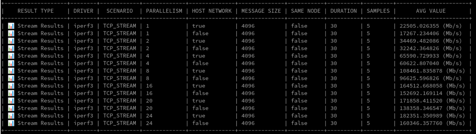
At lower parallelism (up to 4 parallel processes), Layer3+4 performed similarly to Layer2/Layer2+3. But once we pushed beyond 4 parallel processes, the throughput with Layer3+4 really took off. We even recorded over 160Gbps for the pod network with 24 iperf3 processes!
The utilization graph in Figure 9 clearly shows both interfaces getting a good workout.

Figure 10 illustrates the impressive raw numbers.
Wrap up
So there you have it, a deeper look into LACP bonding performance on OpenShift. Choosing the right hashing mode clearly depends on your specific workload and tolerance for potential issues like out-of-order packets. Hopefully, this helps you make a more informed decision for your on-premise OpenShift deployments.
