Page
Complete the four phases of the MLOps pipeline
This lesson will walk the user through creating persisted storage via S3, deploying a model to this storage, exposing this model using functionalities in OpenShift AI, then implementing a Python application to consume the model.
To get full benefit from this lesson:
- Complete the Introduction to OpenShift AI learning path.
- Access the Developer Sandbox or an existing OpenShift cluster.
- Access an AWS account.
- Prior knowledge of Python.
In this lesson, you will:
- Store an ML model in object storage, such as AWS S3.
- Deploy the model on OpenShift AI.
- Use Python within a Flash application to connect and send image prediction requests to the deployed model on OpenShift AI.
Step-by-step guide
The MLOps pipeline consists of four phases:
- Create a new workbench and save the trained model.
- Download and push the trained model to the AWS S3 bucket, using the boto package.
- Fetch the model in OpenShift AI.
- Data connections
- Models and model server
- Model server deployment
- Process the prediction with the deployed model.
Let’s dive into each phase.
1. Create a new workbench and save the trained model
To begin, open OpenShift AI. Navigate to Data Science Projects > (your-sandbox-username)-dev > Create workbench.
Follow these steps to create a new workbench and save the trained model:
- Select the TensorFlow image for the workbench notebook.
- Set the container deployment size to Small.
- Click Create workbench.
- Set Cluster storage size to 10Gi.
Figure 1 depicts the appropriate information entered in the fields on the Create Workbench page.
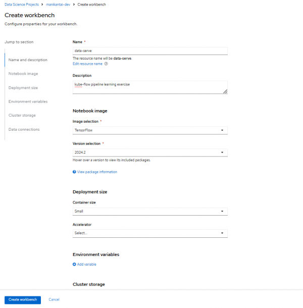
Figure 1: Fill out the fields to create your workbench in OpenShift AI. When the workbench is in the running state, click Open to access the Workbench created (this is a Jupyter notebook).
You will be directed to the Jupyter notebook hosted on OpenShift AI after accepting the permissions. Clone the following GitHub repository into your OpenShift AI workbench-hosted notebook.
From the top menu, click the Git icon.
In the pop-up window, specify the following URL: https://github.com/redhat-developer-demos/openshift-ai.git and navigate to the 3-kubeflow_mlops directory.

2. Download and push the trained model to the AWS S3 bucket using the boto package
For this learning path, we will utilize a pre-trained model called ResNet from ONNX Model Zoo.
To download the model in ONNX file format, open a new notebook and paste the following code in the Jupyter notebook cell:
! wget https://github.com/onnx/models/raw/main/validated/vision/classification/resnet/model/resnet152-v2-7.onnx?download=true -O /opt/app-root/src/image_classification_model.onnxCreate a bucket in AWS S3 and replace
<s3-bucket-name>with its name in the following snippet. Update your AWS credentials and region in the following snippet and execute to push the model to the AWS S3 bucket:import boto3 # Replace with your AWS access key ID and secret access key AWS_ACCESS_KEY_ID = 'Access_Key' AWS_SECRET_ACCESS_KEY ='Secret-Key' # Optional: Specify the AWS region where your S3 bucket resides AWS_REGION = 'ap-south-1' # Example region # Create an S3 client object s3_client = boto3.client('s3', aws_access_key_id=AWS_ACCESS_KEY_ID, aws_secret_access_key=AWS_SECRET_ACCESS_KEY, region_name=AWS_REGION) # s3_client = boto3.client('s3') s3_client.upload_file( Filename='/opt/app-root/src/image_classification_model.onnx', Bucket='<s3-bucket-name>', Key='models/image_classification_model.onnx' )Check your S3 bucket in your AWS account to verify that your bucket lists the model, as shown in Figure 2.
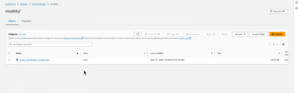
Figure 2: The AWS S3 bucket lists the model.

3. Fetch the model in OpenShift AI
Access the OpenShift AI dashboard within your cluster to initiate preparations for model retrieval.
Data connections
Incorporating a data connection into your project enables you to establish links between data inputs and your workbenches. For handling extensive datasets, consider storing data in an S3-compatible object storage bucket to prevent local storage depletion.
Additionally, you can link the data connection with an existing workbench lacking a connection. This facilitates seamless data access and management within your project workflow.
Follow these steps to create the data connections:
- Select Data Science Projects from the left-hand menu.
- Select the previously used project to create the workbench.
- Click the Connections tab and then the Create Connection button.
- Select S3 compatible object storage - v1 from the Connection Type dropdown.
- Enter the details for the data connection name.
- Enter the access key and secret key of your AWS account.
- Enter the endpoint of the AWS S3 bucket. Based on your region, add the endpoint using this list in the AWS documentation.
- Specify the region where the S3 bucket is located.
- Specify the name of the bucket.
- Click Add data connection to save the connection.
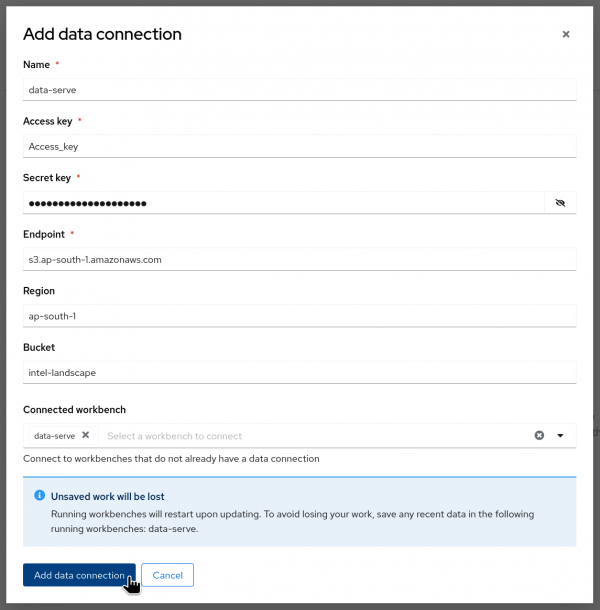
Figure 3 shows the fields with the appropriate information entered.

Figure 3: Create data connections.
Models and model server
Next, deploy a trained data science model for serving intelligent applications. This model will be deployed with an endpoint, enabling applications to send requests for processing. To accomplish this, follow these steps:
- From the left menu, select Data Science Projects.
- Select the project that was used previously to create the workbench.
- Click the Models tab.
- Click Add Model Server.
- Specify the name of the model server.
- Select OpenVINO Model Server as the serving runtime from the dropdown menu.
- Set the Model Server Replicas to 1. Depending on your requirements, you can adjust the number of replicas.
- Define the resource allocation per replica. The model server size will be set to small for this learning path.
- Check the Model route box. This provides an external access domain URL to reach the model server.
- Depending on your security compliance requirements, select whether to use Token authentication. For this learning path, we will not use tokens, so uncheck the box for Require token authentication.
- Click the Update button to finalize the configuration.
Figure 4 shows the fields filled out with the necessary information for configuring the model server.
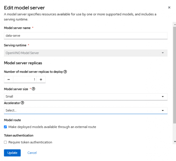
Figure 4: Create the model server.

Deploy the model server
Within the Models and model servers section, you will find the recently created model server listed, as shown in Figure 5.
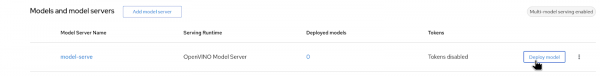
Click the Deploy model button located in the row of the newly created model server.
After clicking the button, a form will pop-up.
Fill out this form according to the following requirements for this learning path:
Specify the name of the model server.
- Choose the ONNX-1 framework from the dropdown menu of the model framework.
- In the Source model location section, select the existing data connection we just created.
- Choose the name of the data connection from the dropdown menu, which we created earlier.
- Add the path of the model under the AWS S3 bucket.
- Click the Deploy button to initiate the deployment process.
Figure 6 is an example of a completed form.
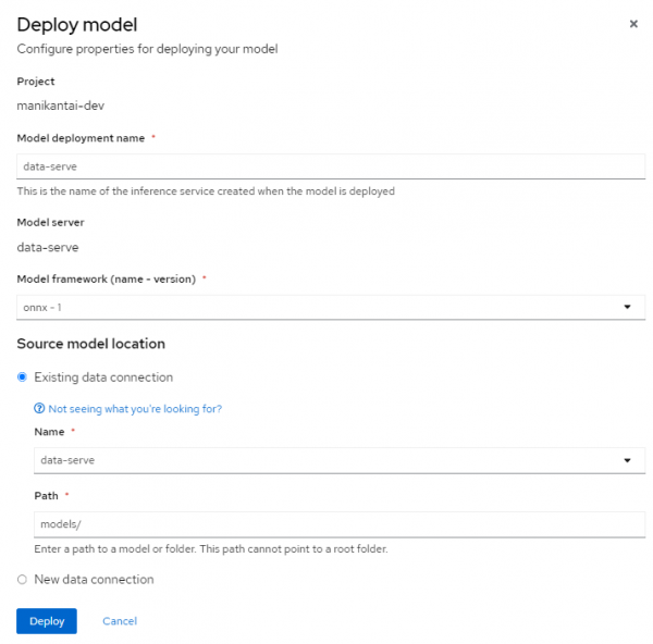
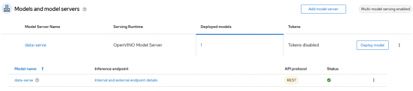
Figure 6: Fill out this form to deploy the model. Upon deployment, ensure that the status of the deployed model server is green, as shown in Figure 7.

Figure 7: The status indicates the model successfully deployed.

4. Process the prediction with the deployed model
For image prediction using the deployed ONNX model on OpenShift AI, copy the external inference endpoint from the listed deployed model (for use later **), as shown in Figure 8.

The following code implements a Flask application that allows users to upload an image and process it with the model we configured earlier.
Replace <insert_inference_url> with the URL of your inference endpoint in the following code:
! pip install flask opencv-python
from flask import Flask, request, render_template
import requests
import json
import numpy as np
import cv2
app = Flask(__name__)
# Function to preprocess image (replace this with your actual preprocessing function)
def preprocess_image(img):
    # Resize image to minimum size of 256x256 while maintaining aspect ratio
    min_size = min(img.shape[:2])
    scale_factor = 256 / min_size
    new_size = (int(img.shape[1] * scale_factor), int(img.shape[0] * scale_factor))
    img_resized = cv2.resize(img, new_size)
    # Crop 224x224 from the center
    center_x = new_size[0] // 2
    center_y = new_size[1] // 2
    half_crop = 112
    img_cropped = img_resized[center_y - half_crop:center_y + half_crop, center_x - half_crop:center_x + half_crop]
    # Normalize pixel values
    mean = np.array([0.485, 0.456, 0.406]) * 255
    std = np.array([0.229, 0.224, 0.225]) * 255
    img_normalized = (img_cropped - mean) / std
    # Transpose image from HWC to CHW layout
    img_transposed = np.transpose(img_normalized, (2, 0, 1))
    return img_transposed
def load_image(image_path):
    return cv2.imread(image_path)
# Function to convert image data to flat array
def image_to_flat_array(image_data):
    return image_data.flatten().tolist()
# Function to convert image data to JSON format
def image_to_json(image_data):
    return json.dumps({"inputs": [{"name": "data", "shape": [1, 3, 224, 224], "datatype": "FP32", "data": image_data}]})
# Function to load class labels
def load_class_labels():
    with open('imagenet_classes.txt', 'r') as f:
        class_labels = f.read().splitlines()
    return class_labels
# Function to perform inference
def perform_inference(image):
    # Preprocess image
    image_processed = preprocess_image(image)

    # Convert image to flat array and JSON format
    image_flat = image_to_flat_array(image_processed)
    image_json = image_to_json(image_flat)
    # Send request to OpenVINO server
    url = '<insert_inference_url>'
    headers = {'Content-Type': 'application/json'}
    try:
        response = requests.post(url, data=image_json, headers=headers)
        if response.status_code == 200:
            # Parse response
            results = json.loads(response.text)
            # Get class labels
            class_labels = load_class_labels()
            # Get the top-1 prediction
            predictions = np.array(response.json()['outputs'][0]['data'])
            top_prediction_idx = np.argmax(predictions)
            top_prediction_label = class_labels[top_prediction_idx]
            return top_prediction_label
    except Exception as e:
        return "Error: {}".format(e)
@app.route('/', methods=['GET', 'POST'])
def index():
    if request.method == 'POST':
        # Check if the post request has the file part
        if 'file' not in request.files:
            return render_template('index.html', message='No file part')
        file = request.files['file']
        # If user does not select file, browser also
        # submit an empty part without filename
        if file.filename == '':
            return render_template('index.html', message='No selected file')
        if file:
            # Perform inference
            file.save('image.jpg')
            img = load_image('image.jpg')
            result = perform_inference(img)
            return render_template('result.html', prediction=result)
    return render_template('index.html')
if __name__ == "__main__":
  app.run(debug=False, host="0.0.0.0", port=5000)
This is the expected output:
[notice] A new release of pip is available: 23.2.1 -> 24.3.1
[notice] To update, run: pip install --upgrade pip
 * Serving Flask app '__main__'
 * Debug mode: off
WARNING: This is a development server. Do not use it in a production deployment. Use a production WSGI server instead.
 * Running on all addresses (0.0.0.0)
 * Running on http://127.0.0.1:5000
 * Running on http://10.128.66.103:5000
Press CTRL+C to quit
To access the Flask application in your browser, duplicate the playbook URL and append /proxy/5000 after the lab address. This is necessary because the JupyterLab server incorporates a built-in proxy server.
Example URLs
- URL of your workbench (from the browser URL bar)
- The endpoint you copied earlier (**)
Replace the lab section with proxy and specify the port number where the application deployed, as shown in Figure 9.
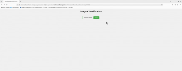
Click Image and choose the Bee.jpeg image. Then, select the Upload button. The Result.html will display the prediction for that image, as shown in Figure 10.

Summary
This learning path demonstrated the deployment of an ML model for image prediction. We first learned to store the model in the object storage (i.e., AWS S3) and deploy it on OpenShift AI. Then, we used Python within a Flask application to connect and send image prediction requests to the deployed model on OpenShift AI.