Train and verify your model

• Now that you have your model, let’s train and test it.

Prerequisites:

• Developer Sandbox account
• General working knowledge of TensorFlow.

In this lesson, you will:

• Train and save your model.
• Test the model.

Train the model

Next, let’s train the machine learning model and measure the training duration. This step utilizes the fit method to train the model on the specified dataset for two epochs while validating its performance on a separate validation set. It applies the class weights to address data imbalance. It also logs the training progress. Then it calculates and reports the total training time.

# Train the model and get performance
import os
import time

start = time.time()
epochs = 2
history = model.fit(
    X_train,
    y_train,
    epochs=epochs,
    validation_data=(X_val, y_val),
    verbose=True,
    class_weight=class_weights
)
end = time.time()
print(f"Training of model is complete. Took {end-start} seconds")

We are training the model for 2 epochs, each epoch consisting of 18750 steps.

The expected output follows:

Epoch 1/2
18750/18750 ━━━━━━━━━━━━━━━━━━━━ 69s 3ms/step - accuracy: 0.8942 - loss: 0.2964 - val_accuracy: 0.9506 - val_loss: 0.2139
Epoch 2/2
18750/18750 ━━━━━━━━━━━━━━━━━━━━ 65s 3ms/step - accuracy: 0.9476 - loss: 0.2355 - val_accuracy: 0.9520 - val_loss: 0.2256
Training of model is complete. Took 134.21636605262756 seconds

Model training is now complete.

Save the model file

The following code snippet converts a Keras model to the ONNX format for compatibility with ModelMesh, a platform for managing machine learning models. Afterwards, it saves the trained model in the model directory:

import tensorflow as tf

# Wrap the model in a `tf.function`
@tf.function(input_signature=[tf.TensorSpec([None, X_train.shape[1]], tf.float32, name='dense_input')])
def model_fn(x):
    return model(x)

# Convert the Keras model to ONNX
model_proto, _ = tf2onnx.convert.from_function(
    model_fn,
    input_signature=[tf.TensorSpec([None, X_train.shape[1]], tf.float32, name='dense_input')]
)

# Save the model as ONNX for easy use of ModelMesh
os.makedirs("models/fraud/1", exist_ok=True)
onnx.save(model_proto, "models/fraud/1/model.onnx")

Confirm the model file creation

List the available models in the model directory using the following command:

! ls -alRh ./models/

The output should include the model's name, size, and date:

./models/:
total 12K
drwxr-sr-x.  3 1004770000 1004770000 4.0K Jul  1 14:43 .
drwxrwsr-x. 13 1004770000 1004770000 4.0K Jul  1 15:52 ..
drwxr-sr-x.  3 1004770000 1004770000 4.0K Jul  1 14:43 fraud

./models/fraud:
total 12K
drwxr-sr-x. 3 1004770000 1004770000 4.0K Jul  1 14:43 .
drwxr-sr-x. 3 1004770000 1004770000 4.0K Jul  1 14:43 ..
drwxr-sr-x. 2 1004770000 1004770000 4.0K Jul  1 14:43 1

./models/fraud/1:
total 24K
drwxr-sr-x. 2 1004770000 1004770000 4.0K Jul  1 14:43 .
drwxr-sr-x. 3 1004770000 1004770000 4.0K Jul  1 14:43 ..
-rw-r--r--. 1 1004770000 1004770000  13K Jul  1 15:53 model.onnx

Test the model

Now we will import specific dependency libraries via the sklearn package so we can handle the pickle models, Matplotlib, and Seaborn to print the diagrams and many more. 

from sklearn.metrics import confusion_matrix, ConfusionMatrixDisplay
import numpy as np
import pickle
import onnxruntime as rt

This loads previously saved objects using pickle. It reads the scalar object from artifact/scaler.pkl and the test data (X_test, y_test) from artifact/test_data.pkl. This is useful for reusing the scaler to transform data or evaluate the model on previously saved test data without retraining the model:

with open('artifact/scaler.pkl', 'rb') as handle:
    scaler = pickle.load(handle)
with open('artifact/test_data.pkl', 'rb') as handle:
    (X_test, y_test) = pickle.load(handle)

Create an ONNX inference runtime session and predict values for all test inputs as follows:

sess = rt.InferenceSession("models/fraud/1/model.onnx", providers=rt.get_available_providers())
input_name = sess.get_inputs()[0].name
output_name = sess.get_outputs()[0].name
y_pred_temp = sess.run([output_name], {input_name: X_test.astype(np.float32)}) 
y_pred_temp = np.asarray(np.squeeze(y_pred_temp[0]))
threshold = 0.95
y_pred = np.where(y_pred_temp > threshold, 1, 0)

The following code snippet calculates the accuracy of predictions by comparing y_test (true labels) with y_pred (predicted labels) and prints the accuracy score. Then it generates a confusion matrix using confusion_matrix from Scikit-learn, visualizes it with a heat map using Seaborn, and displays it using Matplotlib.

This helps in evaluating the model’s performance by showing the number of true positives, true negatives, false positives, and false negatives.

from sklearn.metrics import precision_score, recall_score, confusion_matrix, ConfusionMatrixDisplay
import numpy as np

y_test_arr = y_test.squeeze()
correct = np.equal(y_pred, y_test_arr).sum().item()
acc = (correct / len(y_pred)) * 100
precision = precision_score(y_test_arr, np.round(y_pred))
recall = recall_score(y_test_arr, np.round(y_pred))

print(f"Eval Metrics: \n Accuracy: {acc:>0.1f}%, "
      f"Precision: {precision:.4f}, Recall: {recall:.4f} \n")

c_matrix = confusion_matrix(y_test_arr, y_pred)
ConfusionMatrixDisplay(c_matrix).plot()

The confusion matrix heatmap reveals that the model achieves an accuracy of 97.21%, indicating strong overall performance. It correctly classifies a significant number of transactions, with 181,306 true negatives and 13,107 true positives. These results are illustrated in Figure 1.

The model exhibits high precision, effectively identifying fraudulent transactions with minimal false positives (1,193). However, the recall is lower, with 4,394 false negatives, suggesting that some fraudulent transactions are not detected.

Overall, while the model is accurate and precise, there is room for improvement in capturing more fraudulent activities. The expected output follows:

Eval Metrics: 
 Accuracy: 97.5%, Precision: 0.9511, Recall: 0.7470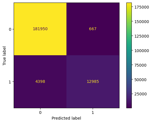

Here is the order of the fields from the transaction details:

1. Distance_from_last_transaction
2. Ratio_to_median_price 
3. Used_chip
4. Used_pin_number
5. Online_order

We are predicting whether a specific transaction (Sally's transaction) is fraudulent and determining the likelihood of fraud.

sally_transaction_details = [
    [0.3111400080477545,
    1.9459399775518593,
    1.0,
    0.0,
    0.0]
    ]

prediction = sess.run([output_name], {input_name: scaler.transform(sally_transaction_details).astype(np.float32)})

print("Is Sally's transaction predicted to be fraudulent? (true = YES, false = NO) ")
print(np.squeeze(prediction) > threshold)

print("How likely was Sally's transaction to be fraudulent? ")
print("{:.5f}".format(100 * np.squeeze(prediction)) + "%")

The model predicts that Sally's transaction is not fraudulent, with a fraud likelihood of only 0.01226%. This suggests the transaction is considered safe based on the model's analysis.

The expected output is as follows:

Is Sally's transaction predicted to be fraudulent? (true = YES, false = NO) 
False
How likely was Sally's transaction to be fraudulent? 
0.01226%

Summary

This learning exercise provided a step-by-step process for developing and evaluating a fraud detection model using TensorFlow and ONNX on Red Hat OpenShift AI. Starting from the Jupyter notebook setup in the Red Hat Developer Sandbox, we configured a TensorFlow workbench and created a neural network tailored for detecting fraudulent transactions. We evaluated model performance with key metrics then converted the model to ONNX format for efficient deployment. Finally, we demonstrated the model’s accuracy with a confusion matrix and conducted prediction tests to verify its fraud detection capabilities.

Learn more

Explore these offerings to learn more about OpenShift AI:

• Introduction to OpenShift AI
• Interactive Image Classification with Jupyter Notebooks on Red Hat OpenShift AI
• Demystify RAG with OpenShift AI and Elasticsearch