Configure and execute an experiment

Now that you’ve created your workbench and accessed the Jupyter notebook, we can move on to loading your Python dependencies and dataset to build your model.

Prerequisites:

• Developer Sandbox account.
• General working knowledge of TensorFlow.
• The workbench set up as detailed in the previous lesson.

In this lesson, you will:

• Install Python packages.
• Load the dataset.
• Build a model.

Install Python dependencies

In this learning path, we will use a sklearn model to create, train, and make predictions from the trained model. We will also handle model saving locally. Before saving, we'll save the model in pickle format and convert it to an ONNX model, as shown in the code snippets that follow. This approach ensures that our model is both efficient and compatible with various deployment environments.

We’ll perform all of the following code steps by executing them in cells in the workbench created in the previous lesson. By cloning the Git repo, you can navigate into the repo directory in the file browser on the left side. Then go into the subdirectory for lesson 4 and click the predefined workbenches (Figure 1).

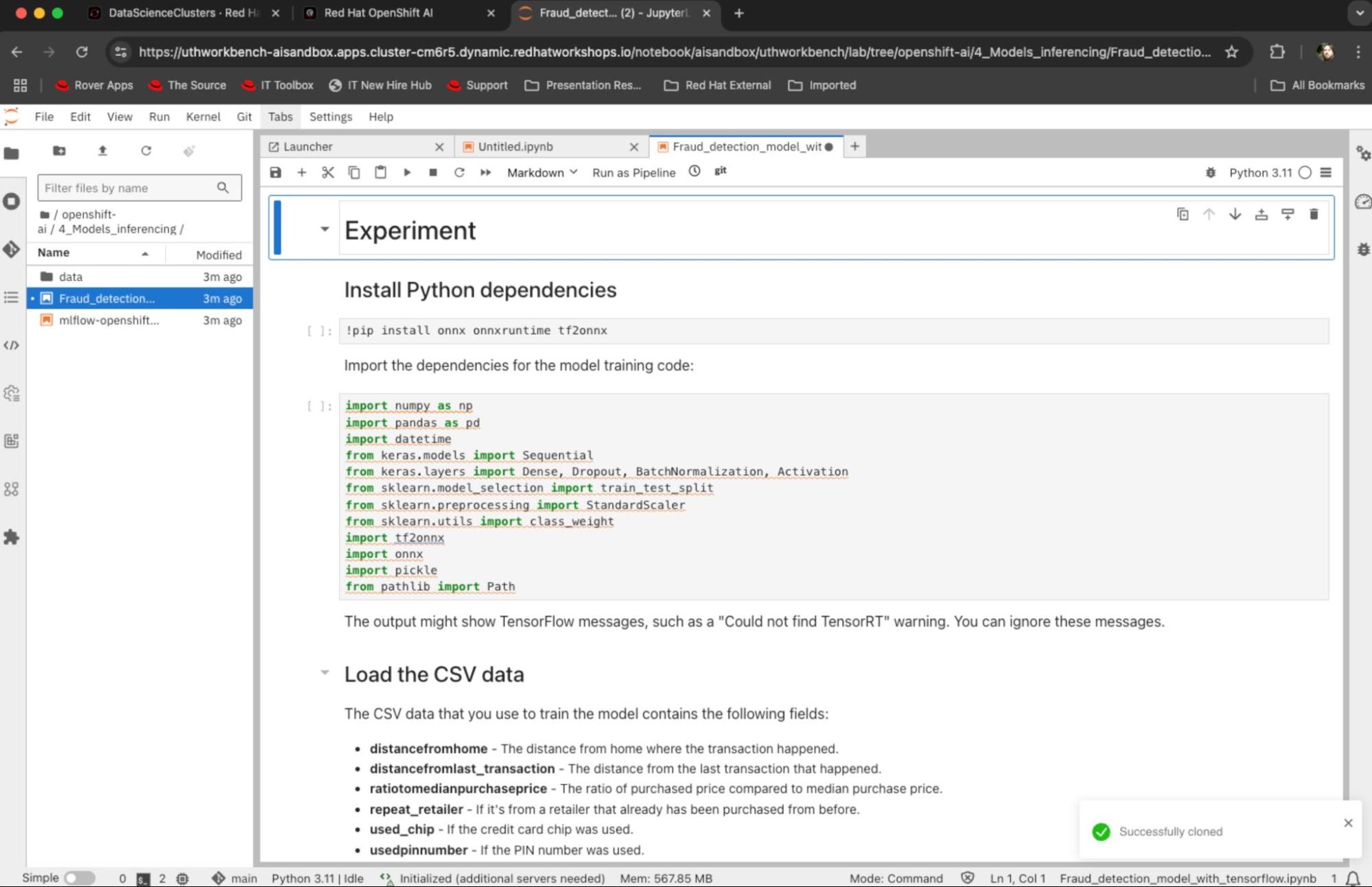
Start by executing the following command to install the required Python packages:

!pip install onnx onnxruntime seaborn tf2onnx

The expected output is as follows:

Collecting onnxruntime
  Downloading onnxruntime-1.18.1-cp39-cp39-manylinux_2_27_x86_64.manylinux_2_28_x86_64.whl (6.8 MB)
     ━━━━━━━━━━━━━━━━━━━━━━━━━━━━━━━━━━━━━━━━ 6.8/6.8 MB 70.9 MB/s eta 0:00:00a 0:00:01
Collecting seaborn
  Downloading seaborn-0.13.2-py3-none-any.whl (294 kB)
     ━━━━━━━━━━━━━━━━━━━━━━━━━━━━━━━━━━━━━ 294.9/294.9 kB 313.6 MB/s eta 0:00:00

The imported libraries and modules facilitate various tasks in machine learning and data processing. NumPy and Pandas handle numerical and data manipulation, while Keras provides tools for building and training neural networks. Scikit-learn aids in data preprocessing and model evaluation. The tf2onnx and ONNX allow model interoperability between frameworks. Pickle is used for object serialization, and Path simplifies file path operations.

import numpy as np
import pandas as pd
import datetime
from keras.models import Sequential
from keras.layers import Dense, Dropout, BatchNormalization, Activation
from sklearn.model_selection import train_test_split
from sklearn.preprocessing import StandardScaler
from sklearn.utils import class_weight
import tf2onnx
import onnx
import pickle
from pathlib import Path

Load and process the dataset

We will now process data for a fraud detection model by extracting specific features and labels from training, validation, and test datasets. The process scales input features to zero mean and unit variance using StandardScaler, fitting the scaler only on the training data to avoid data leakage. It saved the test data and scaler object as artifacts (.pkl files) for future use. Additionally, it computes class weights to address dataset imbalance, giving higher importance to fraudulent transactions during model training:

# Set the input (X) and output (Y) data. 
# The only output data is whether it's fraudulent. All other fields are inputs to the model.
feature_indexes = [
    1,  # distance_from_last_transaction
    2,  # ratio_to_median_purchase_price
    4,  # used_chip
    5,  # used_pin_number
    6,  # online_order
]
label_indexes = [
    7  # fraud
]
df = pd.read_csv('data/train.csv')
X_train = df.iloc[:, feature_indexes].values
y_train = df.iloc[:, label_indexes].values
df = pd.read_csv('data/validate.csv')
X_val = df.iloc[:, feature_indexes].values
y_val = df.iloc[:, label_indexes].values
df = pd.read_csv('data/test.csv')
X_test = df.iloc[:, feature_indexes].values
y_test = df.iloc[:, label_indexes].values
# Scale the data to remove mean and have unit variance. The data will be between -1 and 1, which makes it a lot easier for the model to learn than random (and potentially large) values.
# It is important to only fit the scaler to the training data, otherwise you are leaking information about the global distribution of variables (which is influenced by the test set) into the training set.
scaler = StandardScaler()
X_train = scaler.fit_transform(X_train)
X_val = scaler.transform(X_val)
X_test = scaler.transform(X_test)
Path("artifact").mkdir(parents=True, exist_ok=True)
with open("artifact/test_data.pkl", "wb") as handle:
    pickle.dump((X_test, y_test), handle)
with open("artifact/scaler.pkl", "wb") as handle:
    pickle.dump(scaler, handle)
# Since the dataset is unbalanced (it has many more non-fraud transactions than fraudulent ones), set a class weight to weight the few fraudulent transactions higher than the many non-fraud transactions.
class_weights = class_weight.compute_class_weight('balanced', classes=np.unique(y_train), y=y_train.ravel())
class_weights = {i : class_weights[i] for i in range(len(class_weights))}

No output is expected here.

Build the model

We define a neural network using Keras with several Dense layers, Dropout layers, and Batch Normalization configured for binary classification. It compiles the model with the Adam optimizer and binary cross-entropy loss, and then prints the model summary using the following model code:

model = Sequential()
model.add(Dense(32, activation='relu', input_dim=len(feature_indexes)))
model.add(Dropout(0.2))
model.add(Dense(32))
model.add(BatchNormalization())
model.add(Activation('relu'))
model.add(Dropout(0.2))
model.add(Dense(32))
model.add(BatchNormalization())
model.add(Activation('relu'))
model.add(Dropout(0.2))
model.add(Dense(1, activation='sigmoid'))
model.compile(
    optimizer='adam',
    loss='binary_crossentropy',
    metrics=['accuracy']
)
model.summary()

The model summary shows a sequential neural network with various layers including Dense, Dropout, Batch Normalization, and Activation. It indicates the output shape and the number of trainable parameters for each layer, with a total of 2593 parameters.

The expected output is as follows:

Model: "sequential"
┏━━━━━━━━━━━━━━━━━━━━━━━━━━━━━━━━━┳━━━━━━━━━━━━━━━━━━━━━━━━┳━━━━━━━━━━━━━━━┓
┃ Layer (type)                    ┃ Output Shape           ┃       Param # ┃
┡━━━━━━━━━━━━━━━━━━━━━━━━━━━━━━━━━╇━━━━━━━━━━━━━━━━━━━━━━━━╇━━━━━━━━━━━━━━━┩
│ dense (Dense)                   │ (None, 32)             │           192 │
├─────────────────────────────────┼────────────────────────┼───────────────┤
│ dropout (Dropout)               │ (None, 32)             │             0 │
├─────────────────────────────────┼────────────────────────┼───────────────┤
│ dense_1 (Dense)                 │ (None, 32)             │         1,056 │
├─────────────────────────────────┼────────────────────────┼───────────────┤
│ batch_normalization             │ (None, 32)             │           128 │
│ (BatchNormalization)            │                        │               │
├─────────────────────────────────┼────────────────────────┼───────────────┤
│ activation (Activation)         │ (None, 32)             │             0 │
├─────────────────────────────────┼────────────────────────┼───────────────┤
│ dropout_1 (Dropout)             │ (None, 32)             │             0 │
├─────────────────────────────────┼────────────────────────┼───────────────┤
│ dense_2 (Dense)                 │ (None, 32)             │         1,056 │
├─────────────────────────────────┼────────────────────────┼───────────────┤
│ batch_normalization_1           │ (None, 32)             │           128 │
│ (BatchNormalization)            │                        │               │
├─────────────────────────────────┼────────────────────────┼───────────────┤
│ activation_1 (Activation)       │ (None, 32)             │             0 │
├─────────────────────────────────┼────────────────────────┼───────────────┤
│ dropout_2 (Dropout)             │ (None, 32)             │             0 │
├─────────────────────────────────┼────────────────────────┼───────────────┤
│ dense_3 (Dense)                 │ (None, 1)              │            33 │
└─────────────────────────────────┴────────────────────────┴───────────────┘
Total params: 2,593 (10.13 KB)
Trainable params: 2,465 (9.63 KB)
Non-trainable params: 128 (512.00 B)

Congratulations. You’ve loaded your Python dependencies and dataset and built your model. In the next lesson, you’ll train, save, confirm, and test your model.