An increasing number of Java applications run in containers. The exact number is hard to determine, because adoption of containers depends upon the market segment and cloud maturity of each particular team or company. However, some data is available—for example, data from New Relic suggests that over 62% of their customers' Java workloads run in containers. Like all data points, this one is an imperfect proxy for the market as a whole, but the report demonstrates that a significant subset of the Java market has already moved to container-based environments. Anecdotal data also tells us that this migration trend is far from over.
Teams using Java need to pay special attention to some aspects of container-based deployments and adopt a couple of best practices. This article focuses on the choice of garbage collector (GC) and how the default choice is based on available CPUs and memory.
Java application lifecycle
The traditional Java application lifecycle consists of a number of phases: Bootstrap, intense class loading, and a warmup with just-in-time (JIT) compilation, followed by a long-lived steady state lasting for days or weeks with relatively little class loading or JIT. This makes sense when we remember that Java started as a server-side technology in an era where JVMs ran on bare metal in data centers.
In that world, cluster scaling involved ordering more physical machines and having them delivered to your data centers, application version upgrades happened perhaps every few months, and application processes measured their uptime in weeks or months. Scalability of Java applications typically focused on scaling up, with the goal to make Java perform efficiently on large multicore machines with large amounts of memory.
This model of deployment for Java apps is challenged by cloud deployments in a few distinct but related ways:
-
Containers might live for much shorter time periods (seconds, in some cases).
-
Cluster sizes might be dynamically readjusted or reconfigured (e.g., through Kubernetes).
-
Microservice architectures tend to imply smaller process sizes and shorter lifetimes.
As a result of these factors, many developers, when migrating their Java applications into containers, try to use the smallest possible containers. This seems to make sense, as cloud-based applications are typically charged by the amount of RAM and CPU they use.
However, there are some subtleties here that might not be apparent to engineers who are not Java specialists. Let's take a closer look.
The JVM as a dynamic execution platform
The JVM is a very dynamic platform that sets certain important parameters at startup time based on the observed properties of the machine that it's running on. These properties include the count and type of the CPUs and the available physical memory, as perceived by the JVM. The behavior of the running application can and will be different when running on differently-sized machines—and this applies to containers too.
Some dynamic properties that the JVM observes at startup include:
-
JVM Intrinsics: Hand-tuned implementations of performance-critical methods that rely upon specific CPU features (vector support, SIMD, etc.)
-
Sizes of internal threadpools (such as the "common pool")
-
Number of threads used for GC
Just from this list, you can see that incorrectly defining the resources needed for the container image can cause problems related to GC or common thread operations.
However, the problem is fundamentally deeper than this. Current versions of Java, including Java 17, perform some dynamic checks and decide on the GC to use ergonomically (automatically) if a GC is not explicitly specified on the command line.
To track down the logic for this, let's look at the OpenJDK source code. Specifically, in the src/hotspot/share/gc/shared/gcConfig.cpp file, you can find a C++ method called GCConfig::select_gc(), which calls GCConfig::select_gc_ergonomically() unless a GC is explicitly chosen. The code for this method is:
void GCConfig::select_gc_ergonomically() {
  if (os::is_server_class_machine()) {
#if INCLUDE_G1GC
    FLAG_SET_ERGO_IF_DEFAULT(UseG1GC, true);
#elif INCLUDE_PARALLELGC
    FLAG_SET_ERGO_IF_DEFAULT(UseParallelGC, true);
#elif INCLUDE_SERIALGC
    FLAG_SET_ERGO_IF_DEFAULT(UseSerialGC, true);
#endif
  } else {
#if INCLUDE_SERIALGC
    FLAG_SET_ERGO_IF_DEFAULT(UseSerialGC, true);
#endif
  }
}
The meaning of this code snippet is somewhat obscured by the C++ macros (which are used everywhere in Hotspot's source), but it basically boils down to this: For Java 11 and 17, if you didn't specify a collector, the following rules apply:
-
If the machine is server class, choose G1 as the GC.
-
If the machine is not server class, choose Serial as the GC.
The Hotspot method that determines whether a machine is server class is os::is_server_class_machine(). Looking at the code for this, you'll find:
// This is the working definition of a server class machine:
// >= 2 physical CPU's and >=2GB of memory
This means that if a Java application runs on a machine or in a container that appears to have fewer than two CPUs and less than 2GB of memory, the Serial algorithm will be used unless the deployment chooses a specific GC algorithm explicitly. This result is usually not what teams want, because it typically causes longer stop-the-world (STW) pause times than G1.
Let's see this effect in action. As an example application, we'll use HyperAlloc, which is part of Amazon's Heapothesys project. This benchmarking tool is "a synthetic workload which simulates fundamental application characteristics that affect garbage collector latency."
We spin up a container image from a simple Dockerfile:
FROM docker.io/eclipse-temurin:17
RUN mkdir /app
COPY docker_fs/ /app
WORKDIR /app
CMD ["java", "-Xmx1G", "-XX:StartFlightRecording=duration=60s,filename=hyperalloc.jfr", "-jar", "HyperAlloc-1.0.jar", "-a", "128", "-h", "1024", "-d", "60"]
The HyperAlloc parameters in use are a heap size of 1GB, a simulation run time of 60 seconds, and an allocation rate of 128MB per second. This is the image we will use for a single core.
We'll also create an image that is identical, except for an allocation rate of 256MB per second to use with a two-core container. The higher allocation rate in the second case is intended to compensate for the larger amount of CPU that is available to HyperAlloc, so that both versions experience the same allocation pressure.
Java Flight Recorder (JFR) allows us to capture a log for the entire duration, which is quite short at 60 seconds, but provides ample time to demonstrate the JVM's overall behavior in this simple example.
We are comparing two cases:
-
1 CPU, 2GB image with 128MB alloc rate (Serial GC)
-
2 CPUs, 2GB image with 256MB alloc rate (G1 GC)
The two GC data points that we want to look at are the pause time and GC throughput (expressed as total CPU expended for performing GC) for the separate cases.
If you would like to explore this example and experiment with your own data, the code for it can be found in the JFR Hacks GitHub repository. The project depends upon JFR Analytics, by Gunnar Morling, which provides an SQL-like interface to query JFR recording files.
Note: In all the graphs that follow, the timestamps of the runs have been normalized to milliseconds after VM start.
Let's start with pause time. Figure 1 shows the total pause time for the two cases.
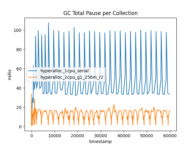
This outcome shows the clear benefit of using G1: All the collections have much shorter pause times. The G1New collections are shorter than Serial's young collections (known as DefNew). However, there are almost three times as many G1New collections as DefNew.
The reason for this leap is that young collections are always fully STW because the allocator threads (the application's threads) tend to have high or unpredictable allocation rates. This means that competition between the GC threads and the allocation threads for CPU is not a winning proposition—it's better to accept an STW pause for young collections and keep them as short as possible.
G1 is not an "all-or-nothing" collector. Because its work is based on regions, it can collect a few young regions to stay ahead of the current allocation rate and then restart the application threads, leading to a higher number of shorter pauses. We will have more to say about the overall effect of this trade-off later.
For the old collections, the effect is even more pronounced: G1Old actually experiences a dip in total pause time, whereas SerialOld experiences a clear spike for the old collections. This is because G1Old is a concurrent collector, and so for the majority of the runtime of the collection, it is running alongside the application threads. In our two-CPU example, while G1Old is running, one CPU is being used for GC and one for application threads.
Figure 2 shows the elapsed time to perform each collection, and contrasts it to the total stop time. This illustrates the concurrent nature of G1Old.
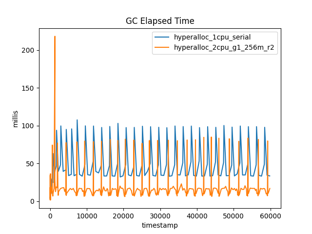
Sure enough, the dips in total pause time that were associated with G1Old have become peaks in elapsed time. It's also apparent to the eye that there are more or less the same number of old GCs whether G1 or Serial is used.
One obvious question that might be asked at this point is: What is the overall cost, in CPU time, of performing GC? Is it possible that, because there are more young G1 collections than young Serial collections, the overall CPU time used by G1 is higher? To answer this question, take a look at Figure 3, which shows the cumulative time spent in GC for the two collectors.
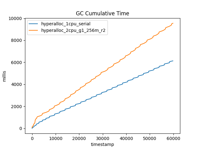
At first glance, it does seem as though G1 uses more CPU than Serial. However, it is worth remembering that the G1 run uses two CPUs and is dealing with twice the allocation rate. So on a per-CPU or per-allocation-GB basis, G1 is still more efficient than Serial.
The overall takeaway is that despite the apparent attractiveness of smaller containers, in almost all cases it is better to run Java processes in containers with two visible CPUs and 2GB of memory and allow G1's concurrent GC to exploit the available resources.
Conclusion, and a look ahead
Having clearly seen the effect in this toy example, there's one major remaining question: How does this effect play out for containers in production?
The answer is that it depends upon the Java version and kernel support in place: In particular—whether a particular kernel API known as cgroups is at v1 or v2.
In the second part of this series, Severin Gehwolf will explain the deep-dive details of exactly how Hotspot detects the container properties and auto-sizes based upon them. You might also want to check out a recent article from Microsoft on containerizing Java applications.
Last updated: December 14, 2023