Page
Measure what matters: benchmarking and evaluation

This lesson focuses on advanced methods for performance optimization, such as benchmarking and evaluation workflows to handle production-grade scenarios, using two open source tools: GuideLLM and lm_eval. You’ll analyze advanced metrics such as time-to-first-token (TTFT) and inter-token latencies across custom load tests. Plus, you will see how to isolate user experience and hardware bottlenecks, validate model accuracy, and make data-driven decisions for LLM deployments.
Prerequisites:
- A free Developer Sandbox account.
- Follow the Getting started instructions in the Prerequisites lesson.
In this lesson, you will:
- Run a real benchmark against your vLLM server and interpret the results using
GuideLLM. - Evaluate model quality with
lm_evalon a standardized task. - Read a published model card data to understand quantization.
- Reason about whether a quantization tradeoff is worth deploying.
How do we evaluate LLMs in production?
Benchmarks and evaluations (evals) are structural processes designed to measure how an LLM performs across the critical tradeoffs of speed, cost, and accuracy.
This relationship creates a “trilemma” among cost, speed, and accuracy. In practice, attempting to maximize any two of these pillars inherently compromises the third. For example, building a system that is both incredibly fast and highly accurate will inevitably demand expensive, high-end compute, while optimizing for low cost and high speed will force a drop in accuracy (Figure 1).
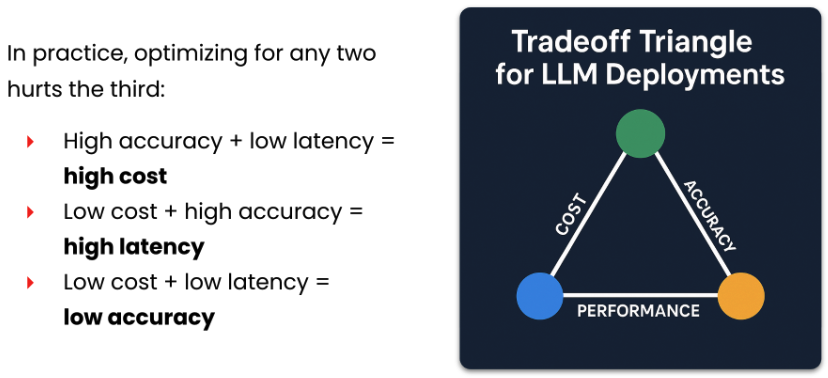
So where does your deployment need to land on this triangle? Without clear measurements, you can’t always answer that question. That’s what this lesson will answer in two distinct ways:
- Evaluations (Evals): Typically focus on validation and accuracy. For example, they utilize specialized datasets or tests to check a model’s capabilities in a variety of domains, from knowledge to reasoning to computer use (for agentic tasks). You can also use evals to ensure stability after a model undergoes optimization techniques like quantization, ensuring that it still outputs high-quality, accurate answers for its targeted tasks.
- Benchmarks: Focus on operational performance and efficiency under load. Tools like GuideLLM are used to simulate realistic real-world traffic patterns (using various concurrency (10 users at the same task) or Poisson (random load) distributions) to stress-test the model's serving engine. This measures fine-grained performance metrics such as latency, throughput (requests per second), and memory/hardware utilization.
These practices are essential for meeting Service Level Objectives (SLOs) and other production metrics because they provide pre-deployment capacity planning, hardware evaluation, and regression testing.
Testing how the system scales when concurrent requests flood the infrastructure allows developers to pinpoint exactly where performance degrades. Ultimately, benchmarks and evals provide the data necessary to guarantee that the deployed model can handle maximum user loads and run efficiently within strict latency and cost constraints without sacrificing the accuracy required by the business.
Complete the setup
In our Jupyter Hub environment, navigate to the benchmarks-evals folder and open the guidellm-lm-eval.ipynb notebook.
We’ll be using the vLLM API key to connect to a running model, which will be used for both the benchmark and accuracy evaluations.
Paste your API key to connect to the Sandbox (Figure 2).
Input:
# Paste your token here (get it with: oc whoami -t)
TOKEN = "YOUR_TOKEN_HERE"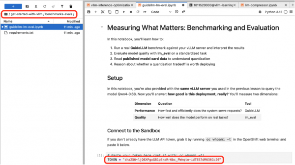
Figure 2: The necessary folder and notebook can be found in the left-hand side menu. Send a quick test request to confirm that everything is working.
Input:
!pip install -q -r requirements.txt

import warnings
warnings.filterwarnings("ignore")

import time, requests, json, os, glob
from openai import OpenAI

VLLM_URL = "https://isvc-qwen3-8b-fp8-predictor.sandbox-shared-models.svc.cluster.local:8443"

client = OpenAI(base_url=f"{VLLM_URL}/v1", api_key=TOKEN)
os.makedirs("outputs", exist_ok=True)

r = requests.get(f"{VLLM_URL}/v1/models",
                headers={"Authorization": f"Bearer {TOKEN}"}, timeout=10)
if r.status_code == 401:
   raise RuntimeError("Token expired — run `oc whoami -t` and paste a fresh one above.")
r.raise_for_status()
MODEL = r.json()["data"][0]["id"]
print(f"Connected — model: {MODEL}")
Output:
Connected — model: isvc-qwen3-8b-fp8
Benchmark with GuideLLM
First we'll create the directory outputs where we'll save the benchmark results. Here is the command we can use to run guidellm. We can run it from the terminal, but here we're running from this code cell using the subprocess module.
Let’s break down the flags we’re passing:
Target VLLM_URL: Points GuideLLM at our local vLLM server. It hits the OpenAI-compatible endpoints.profile synchronous: Sends requests one at a time, waiting for each to finish before sending the next. This gives us a clean baseline of single-request latency, with no batching or queueing in the picture. Other profiles (concurrent, throughput, sweep) ramp up their load to stress-test how the server holds up under traffic.max-requests 10: Caps the run at 10 requests. This is deliberately tiny so that the cell finishes quickly in this environment; a real benchmark would use a few hundred to a few thousand requests, or switch to a time-bounded run with--max-seconds.data prompt_tokens=32,output_tokens=16,samples=32: synthetic workload spec: Each request is ~32 prompt tokens in, ~16 output tokens out, drawn from a pool of 32 pre-generated prompts. Keeping samples>= max-requestsmeans that no prompt repeats, so we don't accidentally inflate prefix-cache hits.output-dir ./outputs: Where GuideLLM writes the JSON report.
We’ll now run the cell. It will take a moment to finish. When it's done, we’ll have a structured benchmark file with per-request distributions, ready to interpret.
GuideLLM saves these results in two formats: JSON and CSV with pre-computed statistics for means, percentiles, min., and max., so that we don't have to calculate them ourselves.
import subprocess
cmd = [
  "guidellm", "benchmark",
  "--target", VLLM_URL,
  "--model", MODEL,
  "--backend-kwargs", json.dumps({"api_key": TOKEN}),
  "--profile", "synchronous",
  "--max-requests", "10",
  "--data", "prompt_tokens=32,output_tokens=16,samples=32",
  "--output-dir", "./outputs",
]
env = os.environ.copy()
env["OPENAI_API_KEY"] = TOKEN
print(f"Running: {' '.join(cmd)}\n")
result = subprocess.run(cmd, capture_output=True, text=True, timeout=600, env=env)
if result.returncode == 0:
  print("Benchmark complete!")
  tail = result.stdout[-2000:] if len(result.stdout) > 2000 else result.stdout
  print(tail)
else:
  print(f"GuideLLM exited with code {result.returncode}")
  print(f"STDOUT:\n{result.stdout[-1000:]}")
  print(f"STDERR:\n{result.stderr[-1000:]}")
Output:
Running: guidellm benchmark --target http://localhost:8000 --model Qwen/Qwen3-0.6B --profile synchronous --max-requests 10 --data prompt_tokens=32,output_tokens=16,samples=32 --output-dir ./outputs
Benchmark complete!
| synchronous | 1.7     | 2.0    | 122.2 | 292.5 | 101.7 | 123.2 | 105.6 | 125.5 |
|=============|=========|========|=======|=======|=======|=======|=======|=======|
ℹ Server Throughput Statistics (All Requests)
|=============|=======|======|=========|==============|===============|==============|
| Benchmark   | Requests             ||| Input Tokens | Output Tokens | Total Tokens |
| Strategy    | Concurrency || Per Sec | Per Sec      | Per Sec       | Per Sec      |
|             | Mdn   | Mean | Mean                                               ||||
|-------------|-------|------|---------|--------------|---------------|--------------|
| synchronous | 1.0   | 1.0  | 0.6     | 26.9         | 9.8           | 34.4         |
|=============|=======|======|=========|==============|===============|==============|
✔ Benchmarking complete, generated 1 benchmark(s)
…   json    : outputs/benchmarks.json
…   csv     : outputs/benchmarks.csv
Interpret benchmark results
Let's now extract from the json files the key numbers:
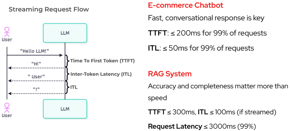
- The time to first token (TTFT): Time to first token measures how quickly the model starts generating a response to minimize perceived waiting time.
- The inter-token latency: Inter-token latency tracks the generation speed of subsequent words to ensure a smooth reading pace.
- The end-to-end latency: End-to-end latency captures the total time required to complete the request to ensure the entire interaction meets strict operational deadlines.
These metrics matter because they directly quantify user experience and system responsiveness for an LLM application (Figure 3).
When we run the cell, the output presents the mean, the 50th, 95th, and 99th percentiles of each metric. This is what we'd put in a report to our team to use or evaluate whether an LLM deployment meets our service-level objectives (SLOs).
Since averages hide outliers, we might notice the p95 (meaning 95% of requests are faster than that value) is worse. We see the same with the p99. This is important because 5 in 100 users could be waiting 20 times longer than usual.
When evaluating a deployment, we always look at the p95 and p99, because if there's a big gap between the mean and the p95, we have tail latency issues, and users will be sure to feel those issues.
with open("outputs/benchmarks.json") as f:
   report = json.load(f)
bench = report["benchmarks"][0]
metrics = bench["metrics"]
n_requests = metrics["request_totals"]["successful"]
print(f"Profile: {bench['type_']}  |  Requests: {n_requests}\n")
display_metrics = {
   "TTFT (ms)":       "time_to_first_token_ms",
   "ITL (ms)":        "inter_token_latency_ms",
   "E2E Latency (s)": "request_latency",
   "Output tokens":   "output_token_count",
}
print(f"{'Metric':<20} {'Mean':>8} {'p50':>8} {'p95':>8} {'p99':>8}")
print("-" * 55)
for label, key in display_metrics.items():
   dist = metrics[key]["successful"]
   p = dist["percentiles"]
   print(f"{label:<20} {dist['mean']:>8.2f} {p['p50']:>8.2f} "
         f"{p['p95']:>8.2f} {p['p99']:>8.2f}")
throughput = metrics["output_tokens_per_second"]["successful"]
req_rate = metrics["requests_per_second"]["successful"]
print(f"\nThroughput: {req_rate['mean']:.2f} req/s  |  "
     f"{throughput['mean']:.1f} output tokens/s")
Output:
Profile: generative_benchmark  |  Requests: 10
Metric                   Mean      p50      p95      p99
-------------------------------------------------------
TTFT (ms)              141.10   122.24   292.45   292.45
ITL (ms)                99.98   101.74   123.18   123.18
E2E Latency (s)          1.64     1.69     2.01     2.01
Output tokens           16.00    16.00    16.00    16.00
Throughput: 0.61 req/s  |  9.8 output tokens/s
Performance benchmarks tell us how fast a deployment is, but not whether the model gives good answers. That's a totally different type of test. We could have the fastest inference server in the world, but if the model's accuracy drops 15% from quantization, then it's not deployable. That's where lm_eval comes in.
Evaluate model quality with lm_eval
lm_eval is a standardized evaluation harness that measures task performance, or how well a model answers on knowledge, reasoning, and coding benchmarks. While GuideLLM asks "how well does this deployment perform?", lm_eval will help us determine "how well this model answers".
We'll point lm_eval at the same running server using the OpenAI completions endpoint, just like we did earlier, and run Hellaswag, a common sense reasoning benchmark. It's the same evaluation that appears on most model cards.
We're using lm_eval’s simple evaluate function on 20 examples to keep it quick, but in production, we would run the full test set once or multiple times.
Run the cell. It'll take a moment to finish, then we’ll review the results.
import lm_eval
os.environ.setdefault("OPENAI_API_KEY", "unused")
TASK = "hellaswag"
print(f"Running lm_eval on {MODEL} via vLLM server ({TASK}, 20 examples)...\n")
results = lm_eval.simple_evaluate(
   model="local-completions",
   model_args=(
       f"model={MODEL},"
       f"base_url={VLLM_URL}/v1/completions,"
       "tokenized_requests=False,"
       "num_concurrent=1"
   ),
   tasks=[TASK],
   limit=20,
)
Output:
Running lm_eval on Qwen/Qwen3-0.6B via vLLM server (hellaswag, 20 examples)...
100%|██████████| 20/20 [00:00<00:00, 2215.22it/s]
Requesting API: 100%|██████████| 80/80 [00:12<00:00,  6.61it/s]
Print out the accuracy metrics. We see a result of 30%, with a standard deviation of around 10%, which isn't the best, but remember that this is a model that could probably fit on a smart fridge.
task_results = results["results"][TASK]
print(f"Model: {MODEL}")
print(f"Task: {TASK}  |  Examples: 20\n")
for metric, value in task_results.items():
   if isinstance(value, (int, float)):
       print(f"  {metric}: {value:.4f}")
Output:
Model: Qwen/Qwen3-0.6B
Task: hellaswag  |  Examples: 20
 acc,none: 0.3000
 acc_stderr,none: 0.1051
 acc_norm,none: 0.3000
 acc_norm_stderr,none: 0.1051
These evaluations give us numerical evidence to make educated model deployment decisions, from deployment performance using GuideLLM, to model accuracy using lm_eval.
We can also use published model card data that's been evaluated by the publisher, before we even get started.
How to read published benchmark data
In a previous lesson, we learned how to quantize a model with llm-compressor. In practice, quantized model publishers include accuracy tables on their model cards so that users can evaluate the tradeoff without running every benchmark themselves.
Here's the accuracy table from the RedHatAI/Qwen3-0.6B-quantized.w4a16 model card—the W4A16 variant of the model we've been working with. The Recovery column shows how much of the base model's accuracy the quantized version retains. Most benchmarks with meaningful base scores show 97–100% recovery, a strong result for a major model size reduction.
Also note that the accuracy of the model using Hellaswag is 43%, which is higher than the 30% we obtained. That's because we only used 20 samples and a single shot.
Category | Benchmark | Qwen3-0.6B | W4A16 (this model) | Recovery |
|---|---|---|---|---|
OpenLLM v1 | MMLU (5-shot) | 42.82 | 39.80 | 93.0% |
ARC Challenge (25-shot) | 32.85 | 30.72 | 93.5% | |
GSM-8K (5-shot) | 1.82 | 2.20 | — | |
Hellaswag (10-shot) | 43.04 | 41.02 | 95.3% | |
Winogrande (5-shot) | 54.54 | 54.62 | 100.1% | |
TruthfulQA (0-shot) | 51.61 | 48.77 | 94.5% | |
Average | 37.78 | 36.19 | 95.8% | |
OpenLLM v2 | MMLU-Pro (5-shot) | 17.25 | 14.27 | — |
IFEval (0-shot) | 62.83 | 55.81 | 88.8% | |
BBH (3-shot) | 4.23 | 1.63 | — | |
Math-lvl-5 (4-shot) | 18.26 | 10.26 | — | |
GPQA (0-shot) | 0.00 | 0.00 | — | |
MuSR (0-shot) | 0.00 | 0.00 | — | |
Average | 17.10 | 13.66 | — | |
Multilingual | MGSM (0-shot) | 19.70 | 19.90 | — |
Reasoning | AIME 2024 | 9.69 | 3.44 | — |
AIME 2025 | 13.13 | 6.98 | — | |
GPQA diamond | 29.29 | 27.78 | 94.8% | |
Math-lvl-5 | 71.60 | 70.60 | 98.6% | |
LiveCodeBench | 12.83 | 8.35 | — |
We now have three sources of evidence:
Source | What it tells you |
|---|---|
GuideLLM | How the deployment performs (latency, throughput, consistency) |
lm_eval | How the model answers (accuracy on a task you ran yourself) |
Model card | How the model performs across many benchmarks, evaluated by the publisher |
When deciding whether to deploy a quantized model, we need both dimensions. An optimization that doubles throughput but drops accuracy by 15% may not be worth it. An accurate model that can't meet latency SLOs isn't deployable either.
Lesson summary
In this lesson, we explored advanced benchmarking and evaluation techniques using GuideLLM and lm_eval to isolate performance bottlenecks and measure model accuracy under production-grade conditions. We analyzed metrics like TTFT variances and standardized evaluation performance to make precise, data-driven decisions for our vLLM deployments.
Learning path summary
In this learning path, we navigated the entire lifecycle of enterprise-ready large language model serving, moving from a base Hugging Face model to a highly optimized production-ready architecture.
By leveraging the llm-compressor library and advanced algorithms (ex., GPTQ), we successfully reduced memory overhead into an efficient format (W4A16) without sacrificing model accuracy.
From there, we got hands-on with vLLM, deploying our models with modern inference optimizations, including PagedAttention, continuous batching, and prefix caching. This allowed us to eliminate memory fragmentation and maximize hardware utilization across both CPU and multi-GPU environments.
We concluded by evaluating model performance and accuracy, stress-testing our deployments under real-world requests using GuideLLM and lm_eval. By analyzing performance metrics, such as TTFT variances and inter-token latencies, we successfully identified potential bottlenecks and verified the precision tradeoffs of our quantized models.
With these configuration strategies and benchmarking insights, we completed the journey, ready to deploy open-source models that are not only highly accurate, but also scalable, cost-effective, and ready for production-grade workloads.
Ready to learn more?
Now that you’ve completed this introduction to vLLM, try these resources:
- Prevent silent failures in your production AI inference stack with end-to-end benchmarking.
- Optimize LLMs with LLM Compressor in Red Hat OpenShift AI
- What is vLLM?
- What are large language models (LLMs)?
- Practical strategies for vLLM performance tuning
- How to deploy and benchmark vLLM with GuideLLM on Kubernetes
- Autoscaling vLLM with OpenShift AI