Optimize a model with LLM Compressor

This lesson provides a hands-on guide to post-training quantization using the llm-compressor library, an optimization tool developed by the vLLM project to compress large language models. The lesson walks through the complete process of reducing a model's operational footprint, for example: use optimization algorithms like GPTQ to compress a model into highly efficient formats (such as W4A16 precision, meaning weights at 4-bit integer while activations stay 16-bit), and run evaluations to guarantee the compressed weights maintain accuracy.

By comparing the base Hugging Face model and quantized model, you’ll go through the steps needed to drastically reduce VRAM requirements and accelerate inference capabilities using vLLM and other serving engines.

Prerequisites:

• A free Developer Sandbox account.
• Follow the Getting started instructions in the Prequisites lesson.

In this lesson, you will:

• Learn how quantization works via full precision and compressed model comparisons.
• Use the llm-compressor library to produce a quantized model at 4-bit weights.
• Test and evaluate the quantized model against the original.

What is LLM Quantization and how does it work?

Quantization is a model compression technique that aims to reduce the memory footprint and speed up the computation of large language models (LLMs) by converting their parameters, such as weights and activations, from higher bit-width floating-point precision (like 32-bit or 16-bit) to lower bit-width representations, like 8-bit or 4-bit integers (Figure 1).

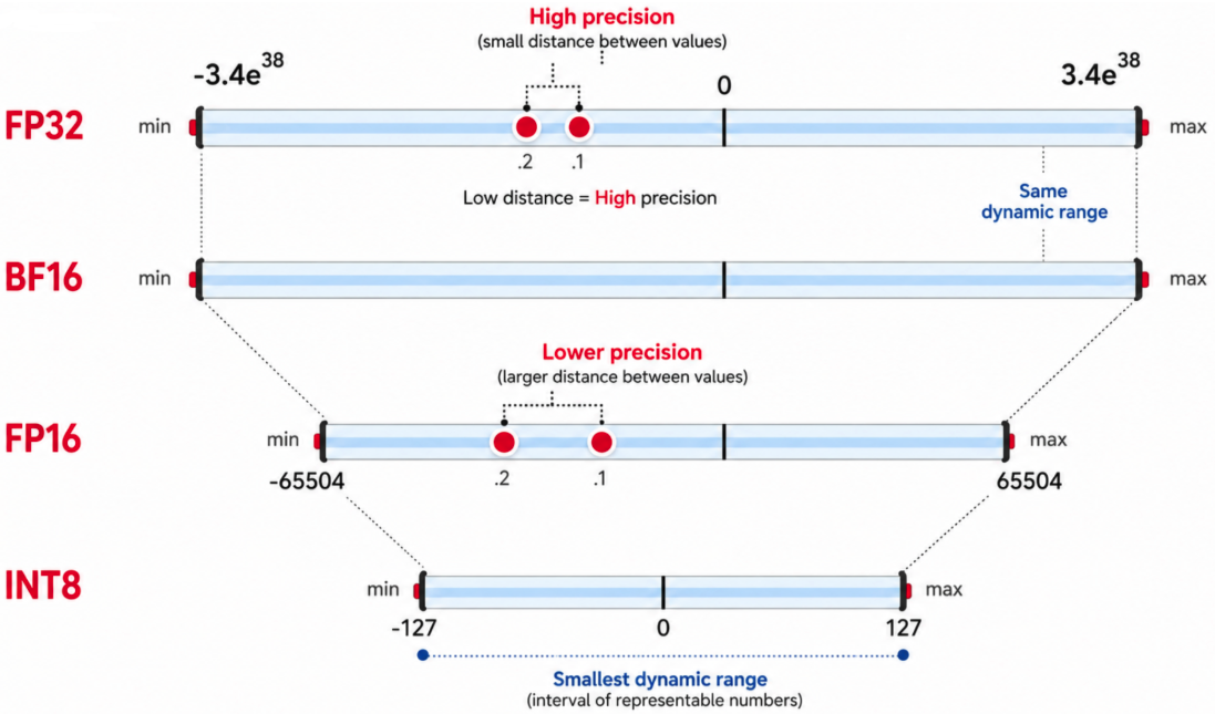
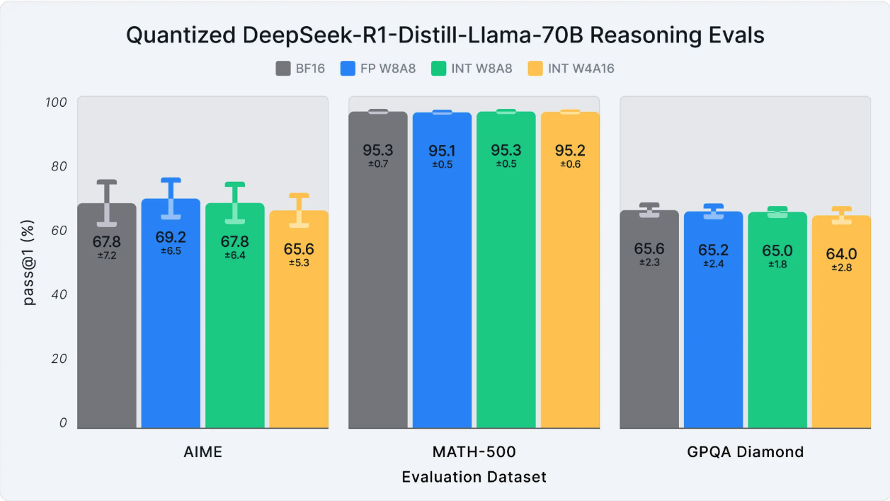
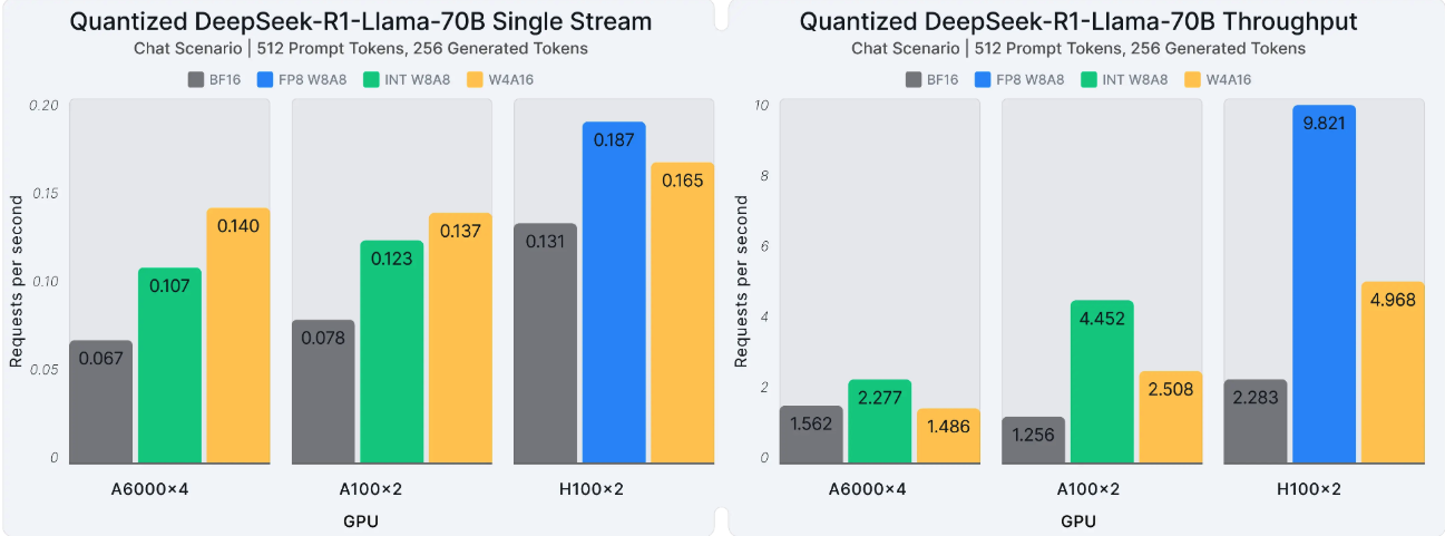
This process functions similarly to reducing the number of colors in an image; it deliberately sacrifices granularity and precision by mapping a vast range of numerical values into smaller, discrete bins. The primary goal is to maximize efficiency and minimize storage requirements while preserving the model’s original accuracy and capabilities as much as possible, as shown with the DeepSeek R-1 quantization below from original precision–BFloat16 to FP W8A8 and below–where leading benchmarks confirm competitive accuracy reasoning while unlocking significant inference speedups (Figures 2 and 3).

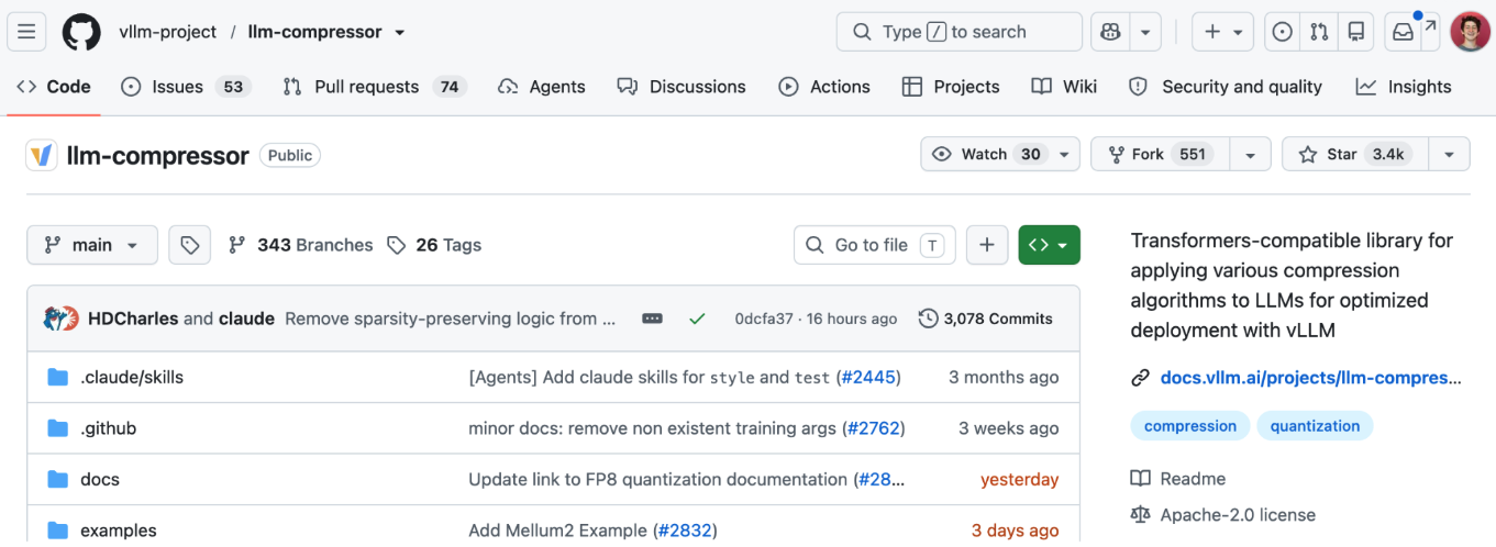
In this lesson, you’ll be using llm-compressor, the production quantization toolkit from the vLLM project. It takes a trained model and reduces precision in a single pass, no retraining required (Figure 4).

The core API is oneshot: you give it a model, a calibration dataset (small sample of real inputs used to minimize quantization error), and a recipe describing how to quantize (e.g., GPTQ, W4A16). It produces a smaller model that can be served directly by vLLM, an LLM inference engine that you'll use in the next lesson.

oneshot(
   model="model-name",           # HuggingFace model ID
   dataset="dataset-name",       # Calibration dataset
   recipe=recipe,                # Quantization configuration
   output_dir="./output",        # Where to save
   num_calibration_samples=512,  # Samples for calibration
   max_seq_length=4096,          # Sequence length
)

The name “oneshot” reflects that this happens in a single pass over calibration data, no retraining required.

Complete the setup

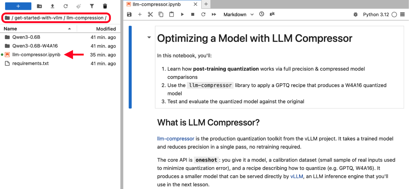
1. In your Jupyter developer environment, open up the llm-compression folder, where you’ll select the llm-compressor.ipynb notebook to work from (Figure 5).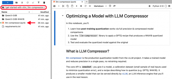

   

2. Next, import our standard libraries, like torch, the Hugging Face transformers for loading models, and tokenizers.

   We’re working with Qwen 3.6B as our base model. It’s small enough to work with in this environment, but it's a capable language model.

   import warnings
   warnings.filterwarnings("ignore")
   import os, gc, math, pathlib
   import torch
   from transformers import AutoTokenizer, AutoModelForCausalLM
   import warnings
   os.environ['TOKENIZERS_PARALLELISM'] = 'false'
   MODEL_DIR = "Qwen3-0.6B"
   OUTPUT_DIR = "Qwen3-0.6B-W4A16"
   print(f"Base model:      {MODEL_DIR}")
   print(f"Quantized model: {OUTPUT_DIR}")

   Output:

   Base model:      Qwen3-0.6B
   Quantized model: Qwen3-0.6B-W4A16

Define the recipe

Next, we’ll need to specify a recipe, which tells LLM Compressor how to quantize. This includes the algorithm to use for quantization, along with the scheme. In other words, how many bits do we want to compress the model to?

We’re using the GPTQ algorithm today, using calibration data to find the optimal quantized values for each weight. Then, we're going for 4-bit weights with 16-bit activations (also known as W4A16), which can lead to a roughly 50% total reduction.

We're targeting linear layers, where the vast majority of parameters live, and ignoring the lm_head, the output layer that maps tokens to vocabulary, so that we keep this compressed model precise.

A recipe could be a list of quantization algorithms, but for our purposes in this lesson, we're using one algorithm:

from llmcompressor.modifiers.quantization import GPTQModifier
recipe = GPTQModifier(
   scheme="W4A16",
   targets="Linear",
   ignore=["lm_head"],
)
print(f"Recipe: {recipe}")

Output:

Recipe: config_groups=None targets=['Linear'] ignore=['lm_head'] scheme='W4A16' kv_cache_scheme=None weight_observer=None input_observer=None output_observer=None observer=None bypass_divisibility_checks=False index=None group=None start=None end=None update=None initialized_=False finalized_=False started_=False ended_=False sequential_targets=None block_size=128 dampening_frac=0.01 actorder=static offload_hessians=False

Quantize the model

To produce the quantized model, we need to import oneshot. It takes the model, some calibration data, and a recipe together to do the compression in a single pass.

from llmcompressor import oneshot
if not os.path.isdir(OUTPUT_DIR):
   oneshot(
       model="Qwen/Qwen3-0.6B",
       dataset="wikitext",
       dataset_config_name="wikitext-2-raw-v1",
       recipe=recipe,
       output_dir=OUTPUT_DIR,
       max_seq_length=4096,
       num_calibration_samples=256,
   )
   print(f"Quantization complete. Model saved to: {OUTPUT_DIR}")

The calibration dataset is used during quantization to ensure the model remains significantly more accurate than it would be using a standard round-to-nearest approach on the weights.

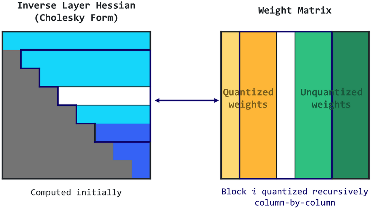
GPTQ and other algorithms run the calibration data through the model to measure how sensitive the output is to each weight. It then finds quantized values that minimize the overall rounding error.

Weights that strongly affect predictions are preserved carefully; less important ones absorb more of the rounding error. The result is a 4-bit model that behaves much closer to the original than what naive rounding would give us (Figure 6).

The dataset parameter specifies what text to use for calibration. Here, we’ll use WikiText-2, a standard benchmark of Wikipedia articles and the same dataset we'll use later for perplexity evaluation.

num_calibration_samples and max_seq_length control that calibration pass:

• Number of calibration samples: How many sequences are run through the model. Having more samples gives a better picture of weight importance, but past a few hundred, the accuracy gains become tiny while runtime keeps growing. 256 is a solid default.
• Max sequence length: The max token length per sample. Longer sequences let the quantizer see how weights behave across realistic context lengths; samples beyond this get truncated.

These parameters help to improve accuracy as we go from default full precision (BFloat16) to Int 4 precision of weights.

Since quantization can take several minutes and benefits from a GPU, we’ve already run it ahead of time and provided the quantized model in the Qwen3-0.6B-W4A16 folder (OUTPUT_DIR).

The if not os.path.isdir(OUTPUT_DIR) check above ensures that we skip re-running quantization when the folder already exists, so you can move straight to evaluation.

Feel free to download this notebook and run this cell yourself to quantize the model on your system!

Compare model sizes

Now we can see what quantization has actually saved us. This cell walks through both model directories, both the original and the compressed ones that we already have in our environment, and then prints a comparison. We’re saving about 50% in just the size of the model.

We might expect a 75% reduction since we went from 16-bit to 4-bit weights (4x smaller), but the actual reduction is 42%. The reason: only the linear layer weights are quantized to Int4. The rest of the model (including the LM head and normalization layers) stays at higher precision.

So the 4x compression applies to the bulk of the parameters (the linear layers, which dominate the model), but the unquantized pieces pull the overall reduction down to ~42%. This ratio improves with larger models, where linear weights make up an even bigger share of total size. A 70B model quantized the same way gets much closer to the theoretical 4x.

def folder_size(path):
   p = pathlib.Path(path)
   if not p.exists():
       return 0
   return sum(f.stat().st_size for f in p.rglob("*") if f.is_file())
def format_size(nbytes):
   if nbytes < 1024**2:
       return f"{nbytes/1024:.1f} KB"
   if nbytes < 1024**3:
       return f"{nbytes/1024**2:.1f} MB"
   return f"{nbytes/1024**3:.2f} GB"
size_orig = folder_size(MODEL_DIR)
size_q = folder_size(OUTPUT_DIR)
reduction = (1 - size_q / size_orig) * 100 if size_orig > 0 else 0
print("Model Size Comparison")
print("=" * 45)
print(f"Original (BF16):    {format_size(size_orig)}")
print(f"Quantized (W4A16):  {format_size(size_q)}")
print(f"Reduction:          {reduction:.0f}%")

Output:

Model Size Comparison
=============================================
Original (BF16):    1.41 GB
Quantized (W4A16):  835.3 MB
Reduction:          42%

Test both models

Smaller model sizes are only useful if the model still works, so let's do a comparison of both using the same prompt. We’ll start with the base model, which we'll load in its original weights on CPU, and give it a prompt like: "machine learning is a branch of...".

Let it generate 60 tokens with standard sampling settings. This is our baseline. Once we're done, we'll remove the original model from memory and load in the quantized one.

prompt = "Machine learning is a branch of"
tokenizer = AutoTokenizer.from_pretrained(MODEL_DIR)
base_model = AutoModelForCausalLM.from_pretrained(
   MODEL_DIR, device_map="cpu", dtype=torch.bfloat16,
)
inputs = tokenizer(prompt, return_tensors="pt")
outputs = base_model.generate(
   **inputs, 
   max_new_tokens=60, 
   do_sample=False,
   pad_token_id=tokenizer.eos_token_id,
)
generated = outputs[0][inputs["input_ids"].shape[-1]:]
print(f"Base Model ({MODEL_DIR})")
print(f"Prompt: {prompt}")
print(f"Response: {tokenizer.decode(generated, 
                                   skip_special_tokens=True)}")
#del base_model; gc.collect()

Output:

Base Model (Qwen3-0.6B)
Prompt: Machine learning is a branch of
Response:  artificial intelligence that has gained significant attention in recent years, particularly in the context of the rise of big data and the need for efficient, scalable solutions to complex problems. As the field continues to evolve, the integration of machine learning into various industries is becoming increasingly widespread. However, despite its growing popularity…

Now we'll be using the quantized model with the exact same prompt and generation settings. The only difference is that the model has 4-bit weights instead of 16-bits.

As before, we’ll run the cell and then compare the two outputs. The quantized model should produce output similar to the baseline. It may not be word for word, but it should remain similar to the original. What we see is a huge compression that comes with minimal quality loss, and that’s our goal.

import logging
logging.getLogger("llmcompressor").setLevel(logging.WARNING)
quant_model = AutoModelForCausalLM.from_pretrained(
   OUTPUT_DIR, device_map="cpu", dtype=torch.bfloat16,
)
inputs = tokenizer(prompt, return_tensors="pt")
outputs = quant_model.generate(
   **inputs, 
   max_new_tokens=60, 
   do_sample=False,
   pad_token_id=tokenizer.eos_token_id,
)
generated = outputs[0][inputs["input_ids"].shape[-1]:]
print(f"Quantized Model ({OUTPUT_DIR})")
print(f"Prompt: {prompt}")
print(f"Response: {tokenizer.decode(generated, 
                                   skip_special_tokens=True)}")

Output:

Compressing model: 196it [00:00, 3156.34it/s]
Quantized Model (Qwen3-0.6B-W4A16)
Prompt: Machine learning is a branch of
Response:  artificial intelligence that focuses on the development of algorithms and models that can learn from data to make predictions or decisions. It has become increasingly popular in various fields, including healthcare, finance, and marketing. However, the field is still in its early stages, and there are many challenges that need to be addressed…

Calculate and compare perplexity

Side-by-side output text gives us an intuition about quality, but now we need a number. That's where perplexity comes in: a standard metric for language models that measures how well the model predicts text. Lower is better, and if quantization has degraded the model, then perplexity will be noticeably higher.

Here we define a calculate_perplexity function that takes a chunk of text from the WikiText-2 test set, slides a window across it, and at each position computes the cross-entropy loss between the model's predicted next-token distribution and the actual next token.

Essentially, it tells us how surprised the model is by the token that actually came next. Exponentiating the average loss gives us perplexity.

Each window moves forward by stride tokens and overlaps with the previous one. The sliding window with stride lets us evaluate long text without feeding it all in at once, and while still giving each token a reasonable amount of context.

1. Load the test split: the same dataset family as calibration, but this time there is a held-out portion, so there's no data leakage.

   from datasets import load_dataset
   def calculate_perplexity(
          model, tokenizer, dataset, max_tokens=5000, stride=512):
      encodings = tokenizer(
          "\n\n".join(dataset["text"]),
          return_tensors="pt", truncation=True, max_length=max_tokens,
      )
      input_ids = encodings.input_ids
      nlls, prev_end = [], 0
      for begin_loc in range(0, input_ids.size(1), stride):
          end_loc = min(begin_loc + stride, input_ids.size(1))
          trg_len = end_loc - prev_end
          input_slice = input_ids[:, begin_loc:end_loc]
          target_slice = input_slice.clone()
          target_slice[:, :-trg_len] = -100
          with torch.no_grad():
              loss = model(input_slice, labels=target_slice).loss
              nlls.append(loss * trg_len)
          prev_end = end_loc
      return math.exp(torch.stack(nlls).sum() / prev_end)
   test_data = load_dataset("wikitext", "wikitext-2-raw-v1", split="test")
   print(f"Loaded {len(test_data)} test samples")

   Output:

   Loaded 4358 test samples

2. Compute perplexity for the quantized model first, since it's already in memory.

   It'll take a moment, as we're running the full test data through the model. Once it's done, we'll clean the model from memory to test the base model.

   quant_ppl = calculate_perplexity(quant_model, tokenizer, test_data)
   print(f"Quantized perplexity: {quant_ppl:.2f}")

   Output:

   Quantized perplexity: 35.48

3. Compute the base model’s perplexity on the same test data. It gives us a reference point.

   base_model = AutoModelForCausalLM.from_pretrained(
      MODEL_DIR, device_map="cpu", dtype=torch.bfloat16,
   )
   base_ppl = calculate_perplexity(base_model, tokenizer, test_data)
   print(f"Base perplexity: {base_ppl:.2f}")

   Output:

   Base perplexity: 32.79

4. Compare the perplexity of the models and review the calculation output.

   print("Perplexity Comparison")
   print("=" * 40)
   print(f"Base (BF16):       {base_ppl:.2f}")
   print(f"Quantized (W4A16): {quant_ppl:.2f}")
   print(f"Difference:        {quant_ppl - base_ppl:+.2f} ({(
      quant_ppl/base_ppl - 1)*100:+.1f}%)")

   Output:

   Perplexity Comparison
   ========================================
   Base (BF16):       32.79
   Quantized (W4A16): 35.48
   Difference:        +2.70 (+8.2%)

Finally, we have the comparison between base perplexity and quantized perplexity, side by side. A small increase is completely expected. We went from 16-bit weights down to 4-bit.

The question is whether the increase is acceptable for our use case. For most production deployments, a few percent increase in perplexity is well worth the reduction in model size and the infrastructure savings that come with it.

Summary

In this lesson, we learned how the oneshot API applies post-training quantization. We compared model sizes and saw the concrete reduction from the base model to quantization with 4-bit weights and 16-bit activations. We tested both models on the same prompt to verify that the output still makes sense. Finally, we measured perplexity to put a number on the accuracy tradeoff.

In the next lesson, we'll take a model and serve it with vLLM, setting up the inference server and interacting with it through the OpenAI-compatible API.