Performance analysis involves identifying and resolving application bottlenecks by measuring data like hardware counters, CPU profiles, and traces. These data files are often large (hundreds of megabytes), with CPU profiles containing extensive instruction cost details. Visually inspecting these large files—including zooming into traces in a browser to find patterns and dependencies—is a laborious and error-prone task.
I experimented with Claude to see if the task of performance analysis turns into a rewarding one rather than exhausting. The results were very encouraging. In this article, I discuss how I used Claude to carry out performance analysis using CPU profiles and traces. I consider the new Go Green Tea garbage collector (GC) as the focal code which is evaluated for optimization opportunities using the sweet benchmark suite on POWER10 architecture.
CPU profile analysis
Go offers the capability to generate CPU profiles for a binary using the Go tool pprof. These profiles can identify performance bottlenecks, even down to the assembly instruction level. Claude works on finding suggestions in these hotspots marked by pprof. The top ten routines where most time is spent, in case of the bleve index benchmark, is illustrated below:
go tool pprof BleveIndexBatch100-1212217505-cpu.prof
File: bleve-index-bench
Build ID: 81f203eb5714d9755a42c833024d5f60afd94e03
Type: cpu
Time: 2026-03-10 16:10:56 IST
Duration: 5.40s, Total samples = 15.18s (280.91%)
Entering interactive mode (type "help" for commands, "o" for options)
(pprof) top 10
Showing nodes accounting for 8830ms, 58.17% of 15180ms total
Dropped 208 nodes (cum <= 75.90ms)
Showing top 10 nodes out of 103
  flat  flat%   sum%    cum   cum%
 3170ms 20.88% 20.88%   4260ms 28.06%  runtime.tryDeferToSpanScan
 1100ms  7.25% 28.13%   2970ms 19.57%  runtime.scanObjectSmall
 840ms  5.53%  33.66%    900ms  5.93%  github.com/blevesearch/segment.segmentWords#
 710ms  4.68%  38.34%   7180ms 47.30%  runtime.scanSpan#
 670ms  4.41%  42.75%   2940ms 19.37%  runtime.scanObjectsSmall

 520ms  3.43%  46.18%    970ms  6.39%  github.com/blevesearch/bleve/index/store/gtreap.itemCompare
 520ms  3.43%  49.60%    3610ms 23.78%  github.com/steveyen/gtreap.(*Treap).union
 440ms  2.90%  52.50%    2070ms 13.64%  github.com/steveyen/gtreap.(*Treap).split
 430ms  2.83%  55.34%      450ms  2.96%  runtime.extractHeapBitsSmall
 430ms  2.83%  58.17%     1690ms 11.13%  runtime.mallocgcSmallScanNoHeader
The atomics example
Within the hottest routine runtime.tryDeferToSpanScan, Claude quickly identified a section of code involving atomics that presented significant opportunities for optimization.
The code performs 2 atomic operations per object:
atomic.Load8(): Check if already marked (1.10s from profile)atomic.Or8(): Set the mark bit (690ms from profile)
Total: 1.79s in atomic operations alone
Proposed optimizations
Single atomic test-and-set (Recommended): The atomic.Or8() function in the Go atomic package is limited because it does not return the old value, unlike atomic.Or32(). Due to this limitation, the current implementation must first use Load8 to determine whether the object is already marked. Given that atomic instructions are costly on the PowerPC architecture, Claude suggested an alternative implementation that uses only one atomic instruction Or32.
// Set mark bit with single atomic operation
idx, mask := objIndex/8, uint8(1)<<(objIndex%8)

// Use Or32 on aligned 32-bit word to get old value
byteOffset := uintptr(idx) & 0b11
wordPtr := (*uint32)(unsafe.Pointer(uintptr(unsafe.Pointer(&q.marks[idx])) &^ 0b11))
shift := byteOffset * 8

if goarch.BigEndian {
    shift = 32 - shift - 8
}
oldWord := atomic.Or32(wordPtr, uint32(mask)<<shift)
if (oldWord>>shift)&uint32(mask) != 0 {
    return true  // Already marked
}
Expected savings: ~1.10s (eliminates the separate Load8)
Claude also pointed out that this is exactly the same pattern used in spanScanOwnership.or() (lines 95-110)!
The suggested approach, although seemingly sound, led to a performance regression. This was primarily due to false sharing in the garbage collection process. Multiple threads accessing the heap bookkeeping area caused contention:
- When threads accessed separate bytes within the same 4-byte word, the lock was applied to the entire word, forcing sequential access.
- This issue was corroborated by Claude, which noted the following problems with the implementation:
- False sharing: Using
Or32means four adjacent bytes share the same atomic operation. - High contention: Multiple GC threads marking different objects in the same span compete for the same 32-bit word.
- Cache line bouncing: Each
Or32operation invalidates cache lines across different CPUs. The profile confirmed this:
- False sharing: Using
atomic.Or32: 0.43s to 1.95s (+1.52s)tryDeferToSpanScanitself improved (4.53s to 2.61s), but the cost ofOr32ate all the gains
Even though optimization does not help in the context of garbage collection, it could make a difference in another application when there is not much contention for the same word.
Arithmetic optimization
In the same function tryDeferToSpanScan, Claude also suggested an interesting Power-of-2 division optimization during objIndex calculation.
// For power-of-2 sizes, use shift instead of magic division
elemsize := gc.SizeClassToSize[q.class.sizeclass()]
if isPowerOfTwo(elemsize) {
    objIndex = uint16((p - base) >> log2(elemsize))
} else {
    objIndex = uint16((uint64(p-base) * uint64(gc.SizeClassToDivMagic[q.class.sizeclass()])) >> 32)
}
The performance improvement from this change is limited, as it only benefits programs that handle objects with sizes that are powers of 2. In other cases, an additional condition check is required. Therefore, this suggestion's effectiveness is heavily dependent on specific benchmark characteristics and is not considered generally effective.
Low-Level code analysis
In the biogo-igor benchmark, Claude suggested caching the q.class.sizeclass variable as a potential optimization. When challenged that the compiler should handle such simple peephole optimizations, and subsequently presented with the assembly dump, Claude confirmed the optimization was not being performed. Furthermore, the model was able to pinpoint the likely reason: an atomic call that accessed a portion of the variable, which likely prevented the compiler from applying the optimization.
This shows that Claude can be used to pore over assembly code and glean insights that are easy to miss, given that the assembly format is difficult to read.
Evidence from Assembly (igor.dump lines 70772-70831):
First Access: Computing objIndex (lines 70772-70789)
# Source: objIndex := uint16((uint64(p-base) * uint64(gc.SizeClassToDivMagic[q.class.sizeclass()])) >> 32)

70773→  0x440e3a  MOVZX 0x7f(DX), SI  #① Load q.class from memory (offset 0x7f in DX)
70775→  0x440e3e  SHRL $0x1, SI   #② Compute sizeclass() - shift right by 1
70777→  0x440e41  MOVSX SI, SI    #③ Sign-extend sizeclass result
...
70784→  0x440e4a  CMPQ SI, $0x44  #④ Bounds check: sizeclass < 68?
70785→  0x440e4e  JAE 0x441012    #⑤ Jump if out of bounds
70786→  0x440e54  LEAQ gc.SizeClassToDivMagic(SB), R8  # ⑥ Load array base address
70787→  0x440e5b  MOVL 0(R8)(SI*4), CX   #⑦ Load gc.SizeClassToDivMagic[sizeclass]
70788→  0x440e5f  IMULQ DI, CX           #⑧ Multiply: (p-base) * divMagic
70789→  0x440e63  SHRQ $0x20, CX         #⑨ Shift right 32 → objIndex
Operations:
- Memory load:
q.classfrom offset 0x7f - Computation:
sizeclass()(right shift) - Array access:
SizeClassToDivMagic[sizeclass]
Second Access: In noscan Path (lines 70814-70831)
# Source: gcw.bytesMarked += uint64(gc.SizeClassToSize[q.class.sizeclass()])

70815→  0x440ead    MOVZX 0x7f(DX), CX         # ① Load q.class from memory AGAIN! (same offset 0x7f)
70817→  0x440eb1    TESTL $0x1, CL             # ② Check noscan bit
...
70823→  0x440eb8    SHRL $0x1, CL              # ③ Compute sizeclass() AGAIN! (shift right)
70825→  0x440eba    MOVSX CL, CX               # ④ Sign-extend AGAIN
...
70827→  0x440ec0    CMPQ CX, $0x44             # ⑤ Bounds check AGAIN: sizeclass < 68?
70828→  0x440ec4    JAE 0x440ffa               # ⑥ Jump if out of bounds AGAIN
70829→  0x440eca    LEAQ gc.SizeClassToSize(SB), DX  # ⑦ Load array base address
70830→  0x440ed1    MOVZX 0(DX)(CX*2), CX      # ⑧ Load gc.SizeClassToSize[sizeclass]
70831→  0x440ed5    ADDQ CX, 0x840(BX)         # ⑨ Add to gcw.bytesMarked
Redundant operations:
- Memory load:
q.classfrom offset 0x7f again (line 70815) - Computation:
sizeclass()again (line 70823) - Bounds: Bounds check again (line 70827)
- Array access:
SizeClassToSize[sizeclass](line 70830)
Prioritization of TODO work in the GC for maximum impact
There are several TODO items embedded within comments throughout the GC code. For developers interested in getting their hands dirty working with the garbage collector, using Claude to sift through the TODOs and prioritize them based on impact and difficulty could be very helpful to ensure they can make a meaningful contribution. Once Claude is familiar with the code base and hotspots, it is in a position to give some good leads.
For example, the following is a list that Claude suggested when presented with the profiles of all sweet benchmarks on PowerPC in priority order based on profile hotness and difficulty:
- Filter nil pointers in write barrier fast path
- Batch heap frees to reduce lock contention in reclaim function
- Lift
sweepLockerout of sweepone loop - Improve fractional mark worker scheduling
- Atomic max primitive for RISC-V
- Better distribution of GC work among
workbufs - Unified greying path through wbBuf in write barrier code
- Skip shading new pointers if stack already shaded in write barrier
- Green Tea GC: Batch spanSPMC freeing
Trace file analysis
Trace files are a vital complement to CPU profiles. While CPU profiles indicate where a performance problem is, trace files provide the necessary insights to understand why. Analyzing a trace file is essential for determining if the garbage collector is causing a performance bottleneck. They can be generated by the option go tool trace.
Pattern recognition and guidance
For beginners trying to learn how to view and understand what the trace file is trying to convey, Claude can be a good guide. The trace output contains thousands of compressed time intervals of data as shown in the figure below. These intervals can be zoomed in by the user to view events occurring in the interval in more detail (figure 1). Visually analyzing a trace file in the browser can be exhausting as unless you know what and where to look.
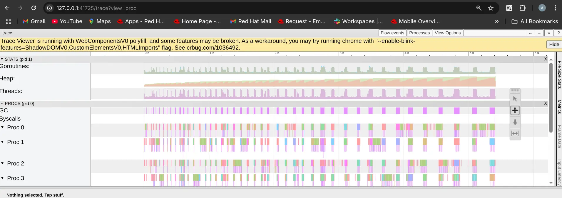
This is where Claude comes handy. When prompted on what patterns to look for, it can provide a nice cheat sheet, as shown below, on patterns to look for at a high level so you can quickly focus on the problematic areas in the trace. Visual patterns to look for:
Good pattern: Dense processor utilization
Continuously busy processors is an indication of efficiency.
P0: ████████████████████████████████
P1: ████████████████████████████████
P2: ████████████████████████████████
P3: ████████████████████████████████
Bad pattern: Idle processors during GC
Gaps during GC marking indicate inefficient work distribution.
P0: ████░░░░░░██████░░░░░░████████
P1: ████████░░░░░░░░██████████████
P2: ░░░░░░░░████████████░░░░░░░░░░
P3: ████████████░░░░░░░░░░░░██████
    ↑ Work imbalance during mark
Bad Pattern: Frequent GC cycles
GC running every 20ms is a very high frequency (expected for igor).
Timeline (1 second view):
GC: █░░░░█░░░░█░░░░█░░░░█░░░░█░░░░
    ↑       ↑       ↑       ↑        ↑      ↑
   20ms     40ms    60ms    80ms     100ms...
Bad pattern: Mark assist gaps
Frequent gaps indicate that the mutator is being throttled.
Application Goroutine:
████░█████░█████░█████░█████░████
      ↑         ↑         ↑         ↑         ↑
      Mark assist pauses (goroutine helping GC)
Good pattern: STW duration
Short STW phases are good.
GC Cycle Zoom In:
STW-Start: █ (< 1ms)
Concurrent Mark: ██████████ (10-20ms)
STW-End: █ (< 1ms)
Bad pattern: Long gcMarkDone
A long gcMarkDone bar indicates a work imbalance.
Mark Phase End:
Workers: ████░░░░ (some finish early)
         ████████ (some still working)
         ████░░░░
gcMarkDone: ░░░░░░░█ (long wait for stragglers)
Pattern recognition cheat sheet
- Dense bars everywhere: Good efficiency
- Frequent vertical lines: Many context switches (bad)
- Gaps during GC phases: Work imbalance
- Regular GC bars < 100ms: Acceptable frequency
- GC bars every 20ms: Too frequent
- Long horizontal blocks: Good, continuous work
- Fragmented blocks: Bad, interrupted work
Extracting GC-related statistics from traces
Sometimes even looking for patterns becomes exhausting due to the sheer size of the trace output. In such cases, you can ask Claude to draw insights from the trace files. For example, in the case of biogo-igor, Claude is able to draw the following conclusions based on the trace statistics:
GC is running frequently:
951 GC cycles in ~20 seconds
= 47.55 GCs per second = One GC every 21ms
- Conclusion: Very high GC pressure
Mark assists indicate mutator throttling:
- 224 mark assist events
- Over 951 GCs = 0.24 assists per GC
- Conclusion: GC marking can't keep up, mutator helping
High allocation rate:
- 179,896 HeapAlloc events in 20s = 8,995 allocations per second
- Conclusion: Allocation-heavy workload
Scheduler churn:
- 130,994 ProcStart/Stop events 15,678 ProcSteal events
- Conclusion: Significant scheduling overhead
Mark termination is expensive:
- gcMarkDone: 181.16ms cumulative
- Across 951 GCs = ~190μs per GC
- Conclusion: Work imbalance in marking phase
It can also give us data points to look for while trying to identify what the problem is. This is useful when we are doing offline analysis and don't have Claude handy.
- GC frequency > 10/sec? Likely GC issue
- Mark assists > 5% of GCs? Marking can't keep up
- gcMarkDone latency high? Work imbalance
- High ProcSteal? Load imbalance
- Many HeapAllocs? Allocation pressure
Parameter tuning
Based on bottlenecks pointed to by trace or CPU profile files, Claude can suggest parameter tuning, which is a favorite among users because it is the least expensive option and doesn't need modification of source code or the Go runtime or compiler, or recompilation of source code. In other words, the gains are "free"!
Some common recommendations given by Claude in the context of GC are shown below. The parameter you choose to tune depends on the bottleneck you encounter in the application.
Tune the GOGC parameter
Lower GOGC to trigger GC more frequently, but with less work per cycle. For example, you could lower it from its default 100 to 50:
export GOGC=50This reduces mark assist by keeping heap growth in check, at the cost of more frequent but shorter GC cycles.
Set Memory limit (requires Go 1.19+)
You can set soft memory limit to prevent excessive heap growth. Adjust based on available memory:
export GOMEMLIMIT=8GiBThis helps the GC pace itself better and reduce mark assist events.
Increase GC workers
If you have spare CPU cores, ensure GOMAXPROCS matches your available cores (this example uses 36, so adjust it for your actual core count):
export GOMAXPROCS=36Comparative analysis
Comparing two trace files to identify performance differences across various phases is a common necessity. Manually comparing trace output in two browser windows is laborious, inefficient and error-prone, especially since traces can contain thousands of data intervals. However, a tool like Claude can effectively highlight these differences as shown below, offering significant value in performance evaluation.
For instance, this capability is crucial when assessing a new feature, such as the Green Tea garbage collector. By generating two traces—one with the baseline GC and one with Green Tea GC—you can compare them to pinpoint areas needing attention.
Also this feature is extremely useful when developing a GC optimization.This capability enables the detection of regressions resulting from the optimization, helping to pinpoint the root cause. Similarly, you can use Claude to compare the CPU profiles of two binaries to analyze the differences.
| Metric | Benchmark: IGOR | Benchmark: KRISHNA | Ratio |
|---|---|---|---|
| Allocations/sec | 9,000 | 175 | 51x |
| GC frequency | 47/sec | 0.1/sec | 470x |
| Mark assists | 224 | 2 | 112x |
| GC CPU overhead | 37% | <1% | 37x |
Multi-trace comparison
Extending this idea forward to more than two benchmarks, we can evaluate the Green Tea GC design at a much higher level. For instance, comparing trace files for all sweet benchmarks, Claude was able to give a high level summary of where Green Tea GC was good at, and where it wasn't.
| Benchmark | GC overhead | Green Tea benefit | Green Tea feature |
|---|---|---|---|
| tile38 | 20-25% | ٭٭٭٭٭ Excellent | Page level tracking eliminates a lot of per-object overhead |
| biogo-igor | 77% | ٭٭٭٭٭ Excellent | Span level batching reduces per object decisions |
| bleve-index | 55% | ٭٭٭٭ Very good | Batch span scanning more efficient than individual object scanning |
| esbuild | 35-40% | ٭٭٭ Good | High parallelism, GC overhead is moderate |
| etcd-STM | 10-15% | ٭٭ Moderate | Main bottleneck is transaction coordination rather than the GC |
| gopher-lua | 10-15% | ٭ Low | GC overhead low |
| etcd-Put | 5% (masked) | ٭ Low | GC overhead low |
| biogo-krishna | 2% | Minimal | Almost non existent GC overhead |
| markdown | 10-15% | Minimal | Almost non existent GC overhead |
In summary, it has been observed based on the patterns seen in sweet benchmarks that Green Tea GC excels when:
- High GC cycle frequency (> 10K cycles)
- Clustered allocations (trees, queues, graphs)
- High mark assist pressure (> 2 assists/cycle)
- Significant time in tryDeferToSpanScan
- High write barrier buffer overhead
Green Tea provides little benefit when:
- Low GC overhead (< 10%)
- Computational bottlenecks dominate
- Sequential allocation patterns
- Large static data with few updates
CPU profiles vs traces: When to use each
Profiles offer instruction-level detail by associating a cost with every instruction. This deep insight helps pinpoint bottlenecks within specific code regions, such as determining what can be improved within a phase like marking or sweeping. Suggestions derived from profiles are typically more immediately actionable.
Traces, conversely, offer a higher-level view, focusing on which phases are most problematic, identifying issues in phase transition, or analyzing how phases are scheduled. Traces can also be very valuable if the application bottlenecks are not CPU bound. If Claude points out that the bottleneck could be in the IO or the network layer, you can focus our efforts on optimizing those layers instead.
Due to their differing input formats, the data and actionable insights provided by profiles and traces are quite different. However, they complement each other effectively in providing a comprehensive view of performance.
In some cases, using both profiles and traces help us converge to the performance issue faster. For example, Claude reports the following in the case of biogo-igor benchmark and suggests adaptive write buffer resizing as a solution.
- CPU profile alone: Shows wbBuf time, but doesn't tell us if 13.56s is normal
- Trace alone: Shows GC frequency, but doesn't show where time goes
- COMBINED:
- Trace shows EXTREMELY high GC frequency (938/sec)
- CPU shows write barrier buffer management is 29.8% of runtime
- Math reveals that the buffer is too small for this allocation pattern
Current limitations
There are limitations to be aware of when using Claude for this kind of analysis.
Architecture-dependent suggestions require validation
Suggestions related to low-level hardware details, such as cache lines, memory layout, SIMD, or ISA, must be validated. The inherent complexity of modern processor architectures can introduce unforeseen dependencies, meaning the assumed performance gains may not materialize. An example exists in the earlier paragraph where Claude suggests using adaptive write barrier buffer resizing without realizing that increasing the buffer size beyond an architecture specific value (cache line size) can actually hurt overall performance.
Short-sighted suggestions miss the bigger picture
Claude may mistakenly identify a "missed optimization", such as a lack of aggressive inlining or loop unrolling, when the compiler intentionally skipped it. This is often done to manage register pressure, demonstrating a trade-off that Claude may have failed to recognize.
Confusion with minimal overhead components (for example, a garbage collector)
When a component like the GC already has minimal overhead or footprint in a specific benchmark, Claude can become confused. For instance, in the gopherlua benchmark, where GC overhead is very low, it incorrectly assumed that the benchmark was not built with Green Tea GC enabled.
To enhance Claude's responsiveness and analytical quality, ensuring suggestions lead to genuine performance gains, we plan to implement an agentic workflow focused on reducing token consumption. Additionally, incorporating specific guardrails using projects.md and skills.md documentation, helps minimize false positives and communicates the functioning of the GC to Claude more effectively, making this experiment worthwhile.
Summary
Claude excels at understanding the binary CPU profile format, including the ability to interpret assembly dumps to identify compiler optimizations. It can suggest simple optimizations though these require subsequent validation and evaluation.
Claude demonstrates a strong grasp of the binary trace format. It can independently parse trace files, filter out events related to garbage collection, and generate scripts for later use. In certain scenarios, Claude can correlate data between traces and CPU profiles. A key capability is its ability to compare two trace or CPU profile files to determine which is superior and provide the rationale. This is useful for identifying regressions or understanding performance differences between versions. This comparative analysis can be extended to multiple files to derive higher-level insights, such as the relationship between memory allocation and GC activity.
Conclusion
Claude is a valuable exploratory tool that augments Go compiler and runtime performance analysis. It helps narrow the focus to likely areas for performance gains, overcoming the manual labor of analyzing large profiles and trace files. It can be used to quickly evaluate a prototype implementation for regressions and improvements as it can compare two profiles and traces, and pinpoint the differences very well. It can also be used over a range of large benchmarks to come up with repetitive patterns and understand the bigger picture of where the implementation excels and where it can be lacking.
As with any AI tool, Claude's suggestions are limited, and architecture-specific recommendations can be inaccurate because providing the complete context isn't always feasible. In some cases, Claude may show confusion when components, like the garbage collector, are already performing well, requiring careful context-setting prompts. You must be mindful of these limitations when utilizing Claude.
Last updated: June 2, 2026