Most retrieval-augmented generation (RAG) tutorials show you how to parse a handful of documents, embed them, and stuff them into a vector database. That's fine for a demomstration. It doesn't hold up when you point it at a real document corpus—thousands of PDF files with complex layouts, tables, and multi-column formatting that simple text extractors mangle.
If you've ever tried to scale a RAG pipeline, you know the frustration: your expensive GPUs sit idle while a single-threaded CPU parser slowly grinds through a mountain of complex PDFs. Running these stages sequentially means you're stuck waiting hours for a job that should take minutes.
A corpus taking hours to parse then sits idle while the system generates embeddings, and not a single vector reaches the database until both stages finish. Organizations end up stuck between "works in a notebook" and "runs in production"—often defaulting to proprietary managed services to close the gap.
We built and tested a distributed ingestion pipeline addressing this directly, processing all three stages in parallel using Ray Data's streaming execution. We show how it works, why streaming changes the performance equation, and how to run it yourself on Red Hat OpenShift AI.
This blog post focuses on the indexing pipeline, the most compute-intensive of the three pipelines making up a production RAG system (indexing, retrieval, and maintenance). Getting indexing right at scale is the foundation everything else depends on.
This post picks up where two earlier pieces left off. A Red Hat blog post, Breaking the RAG bottleneck, introduced the idea of combining Ray Data and Docling for scalable document processing. A follow-up post, Scaling document ingestion with Docling and Ray on Red Hat OpenShift AI, showed how to distribute Docling parsing across a Ray cluster for batch document conversion. Neither of those covered the full pipeline. This post does: from raw PDFs through structured parsing, embedding generation, and vector storage, all running as a single streaming job.
What you'll build
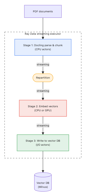
The distributed pipeline has three stages: parse and chunk documents with Docling, generate vector embeddings, and write vectors to a vector database (Milvus in this example). Instead of completing each stage before starting the next, Ray Data's streaming execution overlaps all three. Data flows through the distributed pipeline the way water flows through connected pipes. The first chunks reach the embedding stage while the parser is still working through the document queue. Similarly, the first vectors land in the vector database while embedding is still running, all while Ray Data distributes the workload across multiple worker nodes and actors.
The entire distributed ingestion pipeline starts as a single Python script submitted as a Ray job using the CodeFlare software development kit (SDK). You configure it through environment variables, point it at a directory of PDFs, and it handles distribution, fault tolerance, and stage coordination. A second notebook deploys a large language model (LLM) inference endpoint and demonstrates RAG against the ingested data. Two notebooks, zero external orchestration frameworks, following the three-stage architecture shown in Figure 1.
Why streaming execution matters
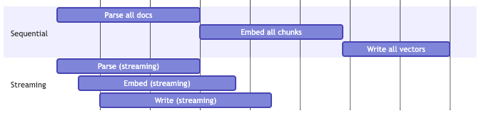
In a conventional pipeline, you would parse every document, collect all the chunks, embed them, and write them to the database. Each stage waits for the previous stage to finish completely. Total wall-clock time is the sum of all three stages.
Ray Data's streaming execution changes this. Each stage processes data in blocks, and downstream stages begin consuming blocks as soon as upstream stages produce them. The practical result is wall-clock time approaches the duration of the slowest stage rather than the sum of all three, as shown in Figure 2.
Streaming execution also keeps memory usage bounded. Only a window of data is in flight at any point. You don't need enough memory to hold every parsed chunk before embedding begins. GPU utilization stays high because the embedding stage doesn't sit idle waiting for parsing to finish. Time-to-first-insert drops from "after all documents are parsed and embedded" to "minutes after the job starts."
The performance difference is structural, not incremental. In sequential execution, a three-stage pipeline taking T1 to parse, T2 to embed, and T3 to write has a total wall-clock time of T1 + T2 + T3. With streaming execution, that total approaches max(T1, T2, T3) because stages overlap. For CPU-intensive parsing workloads, where parsing typically dominates, this can reduce end-to-end time significantly. Throughput also scales linearly with workers. Doubling the number of Docling parsing actors doubles parsing throughput, while the streaming executor keeps downstream embedding and write stages continuously fed instead of waiting for the full parsing phase to complete.
Stage 1: Structure-aware parsing with Docling
The first stage uses Docling to parse PDF documents and the Docling HybridChunker to segment content into chunks. This isn't naive text extraction. Docling understands document structure: tables, headings, lists, and layout elements. When you run a simpler PDF parser, a table might get flattened into a paragraph or split across two chunks, losing the structure that makes it meaningful. Docling preserves that structure, and the HybridChunker respects structural boundaries when creating chunks. That's why parser selection is critical in the indexing pipeline—if the parser can't handle your source documents, nothing downstream will compensate. Docling addresses this for enterprise document types across PDFs, HTML, PPTX, and other formats.
Each parsing actor is implemented as a Ray actor class. During initialization, it loads Docling's machine learning models once and reuses them across every document it processes. Reusing models amortizes the initialization cost, which would otherwise dominate processing time if repeated for every document. The actors run on CPU workers and process documents in configurable batches. Docling parsing is CPU-intensive, so this stage typically has the most actors allocated to it.
Between the parsing stage and the embedding stage, the pipeline repartitions the data. This step spreads chunks evenly across the available embedding workers, preventing hot spots where one worker gets a disproportionate share of the data.
Stage 2: Dual-mode embedding
As shown in Figure 3, the embedding stage supports two execution modes, selectable with a single environment variable.
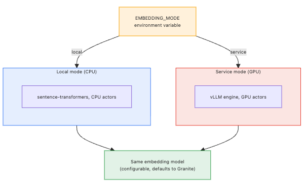
In local mode, sentence-transformers run on CPU actors. No GPU is required. Running in local mode is practical for testing the pipeline, validating your document processing, or running against smaller document sets.
In service mode, the pipeline uses vLLM, a high-throughput model serving engine, through Ray Data's LLM processor API. vLLM is an open source model serving engine designed to deliver high-throughput inference. This runs on GPU workers with automatic batching and GPU memory management. The throughput increase is substantial for production-scale ingestion.
Both modes use the same embedding model. The example defaults to IBM Granite embedding, but any sentence-transformers-compatible model works. Your vectors are identical regardless of which mode produced them. You can develop and test with local mode, then switch to service mode for production runs without changing anything else in the pipeline.
Stage 3: Writing to the vector database
The final stage batch-inserts vectors into a vector database (Milvus) collection. Each write actor manages its own connection to the database and inserts vectors in configurable batches. The actors include retry logic for transient network failures and truncation handling for chunks exceeding field size limits.
Because this stage is input/output (I/O)-bound rather than compute-bound, it rarely becomes the bottleneck. A small number of write actors can typically keep up with the embedding stage's output. The streaming executor keeps them fed with a steady flow of embedded vectors from stage 2.
Resource scheduling and the CPU headroom question
When you configure the pipeline, you decide how many CPU actors to allocate for Docling parsing. Here's the easy-to-miss constraint: Ray Data's streaming executor itself needs CPU resources to coordinate data movement between stages. If you allocate every available CPU to Docling actors, the executor starves and the pipeline stalls. This situation looks like a deadlock, but it's a resource scheduling issue.
To prevent this, you need to leave headroom. The example README documents a sizing approach that reserves a portion of total cluster CPUs for the streaming executor, vector database writers, and GPU worker overhead. When in doubt, start with fewer Docling actors and scale up. The pipeline reports per-stage timing metrics, so you can see which stage is the bottleneck and adjust accordingly.
Best practices
- Start with fewer Docling actors than you think you need and scale up based on per-stage timing. Over-allocating parsing actors starves the streaming executor.
- Use local embedding mode during development and testing. Switch to service mode only when you're ready for production-scale ingestion.
- Monitor per-stage metrics after each run. The pipeline reports timing and throughput for each stage, which makes bottleneck identification straightforward.
- Size your vector database collection before ingestion. Pre-creating the collection with the expected schema avoids runtime errors and lets the write actors batch-insert efficiently.
The technology stack
Figure 4 outlines the full technology stack. At the application layer, Docling handles structure-aware PDF parsing and table extraction, while PyTorch and Transformers power the sentence-transformers library for embedding generation. The vector database (Milvus) stores embeddings and serves similarity searches during retrieval.
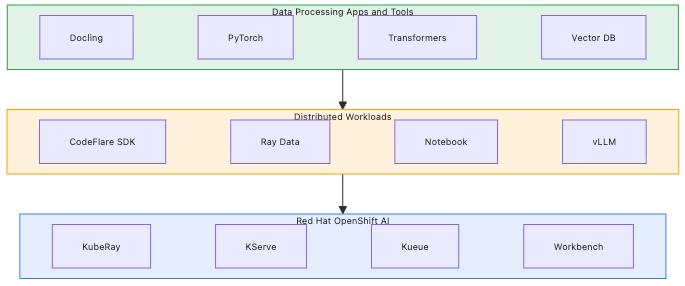
The workloads layer handles distributed execution. Ray Data provides streaming parallel execution across worker pods, orchestrated through the CodeFlare SDK's Python API for RayCluster creation. vLLM serves two roles: GPU-accelerated embedding generation during ingestion and OpenAI-compatible LLM inference for the query path. Notebooks provide the interactive environment for submitting pipeline jobs and running queries.
OpenShift AI provides the platform foundation, and this is where it goes beyond hosting the example. A distributed RAG pipeline like this one creates platform requirements difficult to solve on vanilla Kubernetes: managing Ray cluster lifecycles across diverse CPU and GPU node pools, scheduling GPU resources fairly across teams, serving multiple model endpoints with autoscaling, and giving data scientists a self-service environment to iterate without writing infrastructure YAML.
OpenShift AI addresses these directly. The KubeRay operator manages Ray cluster creation, scaling, and teardown, including ephemeral clusters spinning up for a job and releasing resources on completion. Kueue manages workload queuing, fair-sharing, and quota management across varied CPU and GPU node pools. This is critical when multiple teams compete for GPU capacity, allowing the platform to dynamically schedule Docling CPU workers alongside GPU embedding workers without manual node affinity rules. KServe hosts the embedding and LLM inference endpoints with built-in autoscaling and health monitoring. The CodeFlare SDK lets users create and configure Ray clusters programmatically from notebooks, removing the need for manual cluster provisioning.
As a result, AI engineers can focus on the RAG pipeline logic while the platform handles distributed infrastructure, GPU allocation, model serving, and cluster lifecycle management.
Verifying the pipeline: The query path
The example includes a query notebook validating the retrieval pipeline—confirming the indexed data works for retrieval-augmented generation. It programmatically deploys a language model (Granite 8B in the default configuration, though any compatible model works) as a KServe inference endpoint directly from the notebook using helper functions in the example code. No pre-deployed model is needed, and no manual KServe configuration is required.
The notebook then runs a side-by-side comparison: the same question answered with and without retrieval context. The RAG path embeds the user's question with the same Granite embedding model used during ingestion, searches the vector database (Milvus) for relevant chunks above a similarity threshold, formats the results with source citations, and sends them alongside the question to the LLM. You can see exactly where the model's answer improves with access to your ingested documents, and which source documents contributed to the answer.
This setup is deliberately lightweight. The ingestion pipeline is the focus of this example. The query notebook exists to prove the pipeline's output is usable, not to demonstrate a production query architecture.
What makes this different from typical RAG tutorials
Most RAG examples process documents sequentially on a single machine. They work for a proof of concept but don't address what happens when you have hundreds or thousands of documents. This pipeline is distributed from the start, with streaming execution, structure-aware parsing, and platform-managed infrastructure on OpenShift AI.
The pipeline also includes built-in performance reporting. After each run, you get per-stage timing, throughput metrics, and document processing statistics. These metrics make capacity planning concrete rather than guesswork.
Get started
The full example, including both notebooks, the pipeline script, setup instructions, cluster sizing, and configuration options for both embedding modes, is available in the Red Hat AI examples repository.You'll need an OpenShift AI environment with the KubeRay operator installed and a vector database (Milvus) instance deployed.
Learn more
See how Red Hat OpenShift AI handles the heavy lifting of cluster management and GPU scheduling so you can focus on building.
If you want to understand the foundational concepts before diving into the code, start with the earlier post on breaking the RAG bottleneck with Ray Data and Docling.
For more on the technologies used, see Ray, KubeRay and codeflare-sdk on OpenShift AI, the Docling project, and Ray Data documentation. You can also check out the new e-book, Engineering RAG for the Enterprise.