Many AI projects stall before they begin—before any model is deployed, before the RAG application is running, or before the first chatbot is started. This failure to launch can happen for many reasons, but one of the primary causes is data. Common culprits include a lack of quality data, inaccessible data, and poorly structured or formatted data. Developers spend the bulk of their time on data preparation, and the challenge compounds with "dark data," such as legacy PDFs with complex tables, multi-column layouts, and embedded figures that standard extraction tools mangle or lose. Parsing a few files on a laptop is fine, but scaling to 10,000+ documents without distributed processing can take days.
We built a guided example that combines Docling for structure-aware parsing, with Ray Data for distributed streaming execution, running on Red Hat OpenShift AI. This post covers the architecture, key design decisions, and potential extensions to your batch processing workflow. Also consider reading our blog post on breaking the RAG bottleneck for more details on the business reasons behind this solution.
The stack: High-fidelity parsing at scale
A production ingestion process needs to pair parsing quality with distributed compute. Red Hat OpenShift AI provides the foundation.
Docling
This open source document understanding library and Cloud Native Computing Foundation project uses layout analysis models to recognize tables, code blocks, formulas, and multi-column layouts, producing structured Markdown or JSON.
The quality comes at a cost. Docling loads about 1 GB of machine learning (ML) models at startup and can take 5 to 20 seconds per PDF. Processing 10,000 documents sequentially can take 14 to 55 hours.
Ray Data
This data processing engine and Ray ecosystem component uses a streaming execution model to overlap read, process, and write stages. The framework processes initial documents while subsequent files are still being read. These actor pools amortize Docling's model loading cost by initializing once per actor and processing multiple documents.
KubeRay
This Kubernetes operator and cluster lifecycle management tool uses automated orchestration to govern Ray cluster deployments and autoscaling on OpenShift, handling RayCluster and RayJob custom resources.
CodeFlare SDK
This Python API and cluster management framework uses simplified abstraction layers to convert Kubernetes YAML configurations into Python objects, so you can define cluster specifications, submit jobs, and monitor progress directly from a notebook enviroment.
Prerequisites
Before running the example, you need the following in place:
- Red Hat OpenShift AI with the KubeRay operator installed. The operator manages RayCluster and RayJob custom resources that the example depends on.
- A custom runtime image containing Ray and Docling. The standard OpenShift AI workbench images do not include Docling, so every Ray worker node must run a purpose-built image. A ready-to-build Dockerfile is available in the distributed-workloads repository. It starts from the OpenShift AI Ray CPU base image (
quay.io/modh/ray:2.52.1-py312-cpu) and adds Docling 2.74, pandas, pyarrow, and S3 libraries. Build and push this image to a registry accessible from your cluster, then reference it in the notebook'sClusterConfiguration. - A ReadWriteMany (RWX) PVC mounted on all Ray nodes. Input PDFs are read from this shared volume. The PVC must use a storage class that supports RWX access mode, such as NFS or CephFS.
- A workbench running Minimal Python 3.12 with codeflare-sdk installed. The workbench only submits the RayJob and monitors progress while all heavy processing runs on the RayCluster. No GPU is needed on the workbench.
Architecture
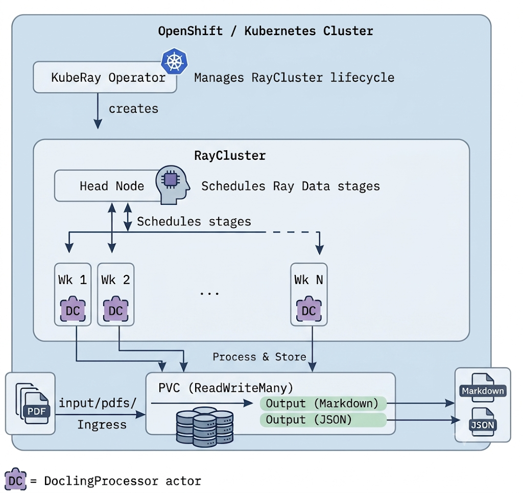
Processing requires either persistent volume claims (PVCs) or S3 or object storage. All Ray workers read from and write to the same ReadWriteMany PVC. By wrapping Docling in a Ray Data map_batches operation, we transform a CPU-bound, single-threaded parsing library into a distributed, multi-node ingestion engine, as shown in Figure 1.
Three-stage processing
The processing script (ray_data_process.py) implements a streaming three-stage process, illustrated in Figure 2:
- Read: Ray Data creates a dataset of file paths on the PVC (not file contents, which keeps memory low regardless of corpus size). The dataset is repartitioned into fine-grained blocks for even distribution across actors.
- Process:
DoclingProcessoractors receive batches of file paths, load Docling's models once, and process many documents. TheActorPoolStrategyscales from a warm pool (min_size) up tomax_sizeunder load. For each PDF, the actor converts via Docling, writes Markdown and JSON to the PVC, and returns per-file metrics. - Report: Results stream back as processing completes. The driver aggregates throughput, error rates, actor distribution, and error details into a performance report.
![Three-stage pipeline showing Read, Process, and Report steps, with a dashed container indicating that Ray Data streaming allows all stages to overlap.]](/sites/default/files/figure-2_18.png)
Because Ray Data streams execution, all three stages overlap. Wall-clock time is dominated by the processing stage, not the sum of all three.
Two deployment patterns
We provide two notebooks using different CodeFlare SDK patterns for different operational needs.
Ephemeral clusters for batch processing
This notebook uses RayJob with ManagedClusterConfig for a complete lifecycle: submit a job, KubeRay creates a cluster, the job runs, the cluster tears down (Figure 3).
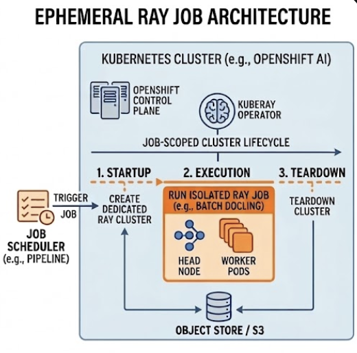
This configuration is best for periodic batch processing, continuous integration/continuous delivery (CI/CD), or any scenario where you want zero idle cost between runs.
Persistent clusters for interactive work
This notebook uses Cluster with ClusterConfiguration to create a long-lived cluster, then submits jobs via the Ray Job Submission Client, as mapped out in Figure 4.
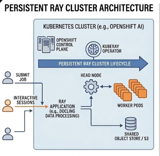
Figure 4: Persistent Ray cluster architecture for interactive workloads.
This setup is best for development, debugging, parameter tuning, or submitting multiple jobs to the same cluster.
Select the deployment pattern that best aligns with your operational requirements and development workflow.
| Operational need | Recommended deployment pattern |
|---|---|
| Nightly batch processing | RayJob |
| First-time setup, tuning parameters | RayCluster |
| CI/CD integration | RayJob |
| Processing different document sets iteratively | RayCluster |
| Production automation | RayJob |
The configuration calculator
Sizing a Ray cluster for Docling means balancing actors per worker, CPUs per actor, memory allocation between Ray's object store and actor heap, and dataset partitioning for even distribution.
The configure.py script encodes these relationships and produces a complete configuration from a few inputs, outputting ready-to-paste code snippets for job submission.
Key formulas:
- Schedulable CPUs per worker =
worker_cpus- 2 (reserves 2 CPUs for Ray's raylet and object store) - Actors per worker =
schedulable_cpus/cpus_per_actor - Max actors =
num_workersxactors_per_worker - Memory per actor = (
worker_memory-object_store) /actors_per_worker(must be >=4 GB; >=6 GB with OCR) - Total blocks =
max_actorsxrepartition_factor(fine-grained blocks prevent straggler effects)
It also validates constraints and warns about low actor memory, straggler risk from oversized blocks, over-provisioned clusters, or batch sizes that exceed files per block.
Example output for 8 workers x 8 CPUs x 16 GB, processing 10,000 PDFs:
- Workers: 8 x (8 CPUs, 16 GB)
- Schedulable CPUs: 6 per worker (2 reserved)
- Actor pool: 8..24 (2 CPUs, approximately 4.8 GB each)
- Estimated time: Approximately 35 min (fast) to 2.3 hr (slow)
Performance characteristics
Each run produces a performance report covering throughput (files/second, pages/second), actor distribution, error and timeout rates, and per-file processing times.
Performance is highly dependent on the hardware, CPU and memory of workers. Sample throughput for standard business PDFs (5 to 20 pages, text-heavy, some tables) and simple Docling configurations includes:
- 8 workers x 8 CPUs: About 4 to 8 files/second (10,000 files in 20 to 40 minutes)
- 4 workers x 8 CPUs: About 2 to 4 files/second (10,000 files in 40 to 80 minutes)
Processing time scales linearly with document complexity. The repartition_factor and per-file timeout settings let you tune for your specific document mix.
Extending for your own environment
We designed this example as a starting point. Common extensions include:
- Different document types. Docling supports DOCX, PPTX, HTML, and images. Change the glob pattern and format options. Docling auto-detects by extension.
- Connecting to S3 instead of PVC. Replace PVC reads/writes with
boto3calls orray.data.read_binary_files("s3://..."). This removes the ReadWriteMany requirement at the cost of network latency per file. - Enabling OCR (optical character recognition). Set
do_ocr = Truein the processing options. Increase memory per actor to 6 GB or more (optical character recognition models add about 2 GB). Use the configuration calculator with--ocrto validate sizing. Expect 2 to 5 times slower processing. - Custom output formats. Docling also supports Doctags and dictionary export. Modify the converter subprocess to call additional export methods alongside Markdown and JSON.
Summary
Combining Docling's parsing accuracy with Ray Data's distributed streaming execution addresses the two core problems in document ingestion: data quality and scale. Subprocess isolation ensures fault tolerance. The configuration calculator removes guesswork from cluster sizing. And two deployment patterns (ephemeral RayJob runs for automation, persistent RayCluster setups for development) let teams match compute strategy to workflow.
Of course, there are scenarios (such as a small set of documents) that might not require the distribution and scalability of Ray, in which case using Docling directly on the documents might be enough.
Red Hat OpenShift AI provides the orchestration and networking to move these workloads from laptop to production with minimal code changes.
Get started
Document ingestion is the front of every retrieval-augmented generation (RAG) and agentic pipeline: the quality and scale of your parsing determines what your models can actually reason over. This example gives you a scale-ready starting point.
Try the guided example
Clone the repository, navigate to the folder red-hat-ai-examples/examples/ray/data/docling, create an OpenShift AI workbench, and run your first batch in under an hour. The notebooks walk you through both deployment patterns, so you can start interactively and move to automated batch jobs when you are ready.
Adapt it to your environment
Point the pipeline at your own document types, switch from PVC to S3, or enable OCR for scanned archives. Use the configuration calculator to size your cluster for your corpus and hardware, rather than guessing at actor and memory settings.
Build it into your AI platform
Structured, scalable ingestion is the foundation for RAG and agentic workloads on Red Hat OpenShift AI. Once your documents are parsed into clean Markdown and JSON, the same platform provides the model serving, tuning, and orchestration to turn that data into production AI applications.
Join the conversation
Questions, improvements, or a document type that breaks in an interesting way? Open an issue or start a discussion in the Red Hat AI community.
References and resources
- Guided example code: Red Hat AI Examples repository on GitHub
- Docling project: Official Docling documentation and resources
- Ray project: Ray framework for scaling Python applications
- KubeRay documentation: Kubernetes operator for Ray clusters
- CodeFlare SDK: Python API for managing Ray clusters on OpenShift
- Breaking the RAG Bottleneck: Scalable Document Processing with Ray Data and Docling: Anyscale blog on Ray Data and Docling for RAG document processing