Let me paint you a picture. You have 16 NVIDIA H200 GPUs spread across 2 nodes. That is, conservatively, several 100,000 dollars of silicon sitting in a data center, connected by RDMA/InfiniBand, running Kubernetes, and serving a large language model. You're living the agentic dream (not really, but it's a great start). Except your time to 1st token (TTFT) is thousands of milliseconds. Your users are waiting seconds before they see anything, not because your GPUs are slow — they're perfectly capable. The issue is that the default inference settings are designed to work safely on any setup, from a single A10G to a 16-GPU H200 cluster. That's like shipping one shoe size for every foot on the planet. It technically fits most people, but nobody is running a marathon in it.
Here is the thing nobody tells you when you buy GPUs: Hardware is only half the battle. The other half — the half that determines whether your inference service feels like a sports car or a 1994 clunker with a misfire — is configuration. And there are a lot of knobs to turn.
What if I told you that on the exact same hardware, with the exact same model, the exact same workload, you could cut latency from a default 995ms down to 304ms TTFT at 23.6 requests per second — and then to 287ms with smarter request routing? That's a 71% reduction in latency with no loss in throughput
I decided to systematically optimize my inference stack. I tested every reasonable architecture, swept dozens of configurations, tuned engine parameters from 1st principles, and measured everything with Prometheus. This post is the story of what I found, and how much performance you are probably leaving on the table right now.
My test setup
I ran all my experiments on a CoreWeave cluster with the following specs:
- GPU: 16x NVIDIA H200 (140 GB HBM3e each)
- Nodes: 2 nodes, 8 GPUs per node
- Interconnect: RDMA / InfiniBand (critical for PD disaggregation)
- Total GPU Memory: 2,240 GB
- Platform: CoreWeave Kubernetes
Software stack
I used llm-d (part of Red Hat AI Inference 3.4) with vLLM v0.18.0 as the inference engine. The full stack runs on Kubernetes with custom endpoint picker (EPP) routing.
Qwen/Qwen3-32B
- Parameters: 32B
- Precision: BF16
- Notes: Dense model, smaller KV heads
RedHatAI/Meta-Llama-3.1-70B-Instruct-FP8-dynamic
- Parameters: 70B
- Precision: FP8
- Notes: Larger model, grouped-query attention, more KV heads
Workload Profile
I deliberately chose a realistic enterprise workload, not the synthetic toy benchmarks you see in most blog posts. Here is what I threw at the system:
- Input sequence length (ISL): 2,000 tokens
- Output sequence length (OSL): 100 tokens
- Concurrent Users: 100
- Prefix cache hit rate: 50% (multi-group, 10 groups)
- Workload type: Enterprise RAG-style: long prompts, short responses
This is the kind of workload you see in enterprise RAG deployments. Users submit long documents or context windows (2,000 tokens of input), and the model generates relatively short responses (100 tokens). With 100 concurrent users and 50% prefix cache overlap, this mirrors a scenario where multiple users are querying against overlapping knowledge bases. If your benchmark uses ISL=256 and OSL=256, I respectfully suggest that your benchmark is lying to you.
Understanding the architecture options
Before I dive into the tuning results, I need to talk about the 2 fundamental deployment topologies for an LLM inference service: Aggregated and prefill-decode (PD) disaggregated. There are sharding techniques, like expert parallelism (EP), which distributes MoE experts across GPUs rather than sharding layers, but EP is a parallelization strategy you can apply with either deployment model. For this post, I focus strictly on the top-level topologies: Aggregated and disaggregated
Aggregated mode
In aggregated mode, every GPU pod handles both prefill (processing the input prompt) and decode (generating output tokens). This is the simple, default deployment. You spin up some number of replicas — each configured with your chosen degree of model parallelism (like Tensor Parallelism) — and let a load balancer throw requests at them.
The advantage is simplicity. No special networking, no KV cache transfer, no coordination. The disadvantage: You're asking each GPU to be good at 2 very different things, simultaneously. Prefill is compute-bound (process 1000s of input tokens in 1 big matrix multiplication), while decode is memory-bandwidth-bound (generate 1 token at a time, reading from KV cache). It's like asking the same person to be both a sprinter and a marathon runner. Some can do both, but most excel at one or the other.
Prefill-decode disaggregated mode
In PD disaggregated mode, you split your GPU pool into 2 groups: Prefill pods (which only process input prompts) and decode pods (which only generate output tokens). After a prefill pod processes the prompt, it transfers the KV cache to a decode pod via NIXL over RDMA/InfiniBand, and the decode pod takes over for token generation.
The advantage: Each pod is optimized for its specific task. Prefill pods can batch aggressively and use their compute capacity fully. Decode pods can maximize memory bandwidth utilization.
The disadvantage: You need RDMA for efficient KV cache transfer, and the split introduces a scheduling problem. How many prefill pods vs. decode pods? Too many prefill pods means your decode phase starves. Too few means users wait longer for that 1st token.
Finding the right P/D split was one of the core challenges I set out to solve. Given my hardware, model, and workload, what is the optimal split?
The great configuration hunt: Qwen3-32B
I started with Qwen3-32B and the stock Red Hat AI Inference 3.4 default templates. No tuning, no parameter changes — just the upstream defaults that ship with llm-d. These defaults are deliberately conservative, because they need to work on everything from a single-GPU dev box to a 64-GPU production cluster. I wanted to see what that baseline looked like on my specific hardware before tailoring anything.
Baseline: Red Hat AI Inference 3.4 defaults
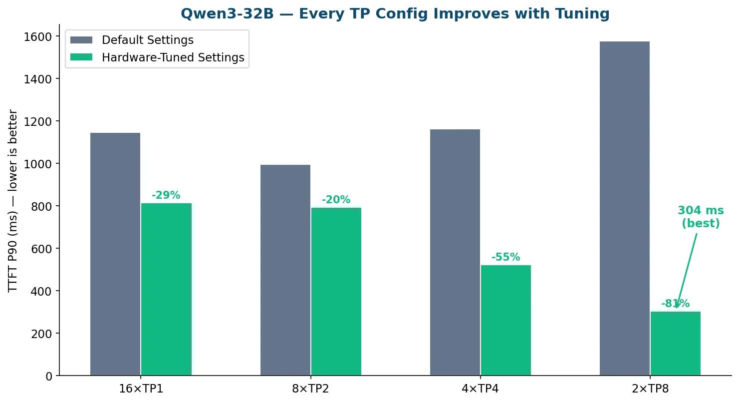
Figure 1 shows what I got with the default templates:
8x TP2
- Architecture: Aggregated
- TTFT P90: 995ms
- Throughput: 24.6 req/s
3P+1D TP4
- Architecture: PD disaggregated
- TTFT P90: 675ms
- Throughput: 22.5 req/s
Almost a full second for TTFT P90 in aggregated mode. The PD configuration was better at 675ms, but still far from great. In interactive LLM benchmarks, 200–300ms TTFT is widely treated as the target threshold for short-to-medium prompts (~2k input sequence length), past which human users register a noticeable delay. At nearly 1,000ms, the initial aggregated baseline was roughly 3x over that interactive threshold.
Of course, massive 20k+ prompt contexts inherently demand longer prefill times, but for a standard 2k workload, sub-300ms was fully achievable.
Not bad, but I knew I could do better. The question was: Which knobs to turn?
Exploring the PD configuration space
I started by testing every reasonable PD split I could think of. With 16 GPUs, there are many ways to divide them between prefill (P) and decode (D) pods at various TP degrees. I ran the full sweep (figure 2).
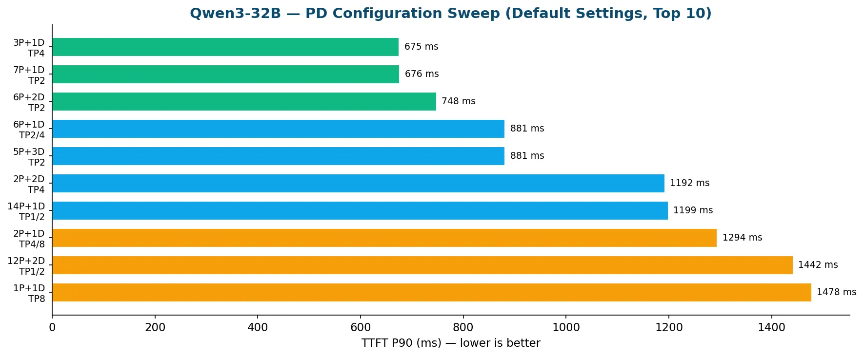
The patterns were clear: More prefill pods consistently reduced TTFT because the prefill phase (processing the full 2,000-token input) is the bottleneck for first-token latency. With more prefill pods, incoming requests are less likely to queue waiting for a prefill slot.
However, there is a sweet spot. Allocating too many GPUs to prefill starves the decode phase and reduces sustained throughput, while allocating too few leads to massive queuing. Evaluating configurations across both lower TTFT and higher throughput revealed which splits achieved the optimal balance.
The default winner was 3P+1D TP4 at 675ms TTFT and 22.5 req/s. But I wasn't satisfied. What if the real gains were not in the P/D split, but in the engine parameters underneath?
vLLM tuning
vLLM has dozens of configuration parameters, but in my extensive testing, 4 parameters consistently had the biggest impact on performance. Let me walk through each, because understanding why they matter is just as important as knowing what to set them to.
gpu_memory_utilization: 0.90 to 0.95
This parameter controls what fraction of GPU memory vLLM is allowed to use. The default is 0.90 — a smart conservative choice that works safely across every GPU from a 24GB L4 to a 140GB H200. But on my H200s, that 10% headroom means 14 GB per GPU sitting unused. That's 14 GB that could be holding KV cache for additional concurrent sequences.
I tuned gpu_memory_utilization to 0.93-0.95. At 0.95, I reclaim an additional 7 GB per GPU compared to the default. Across 8 GPUs, that's 56 GB of extra KV cache — enough to serve 40 more concurrent users before hitting memory pressure The risk? Push it too high and you get out of memory (OOM) errors under peak load.
I found 0.95 to be the sweet spot for H200s with my workloads. It's aggressive enough to matter, but conservative enough to not crash at 3 AM when your on-call engineer is asleep.
max_num_seqs: The most important parameter you've never tuned
This is arguably the most impactful parameter, and the one where I spent the most engineering effort developing a smart formula. The max_num_seqs setting controls how many sequences can run simultaneously on a single engine. Set it too low and your GPU sits idle between batches. Set it too high and you overflow memory or saturate compute.
My formula computes max_num_seqs as the minimum of 4 constraints:
S_activation: How many sequences the GPU can handle based on activation memory (the working memory used during forward passes, distinct from KV cache)S_kv: How many sequences the KV cache can hold given the available memory, model architecture, and sequence lengthS_concurrency: How many concurrent sequences you actually need based on your workload concurrency divided by the number of replicas- A hard cap of 512 to prevent scheduler overhead from dominating
For Qwen3-32B at TP=8, the formula yields max_num_seqs=192. I demonstrate later how wildly different this number is for Llama-70B, and why every model-hardware combination needs its own value.
These are not random numbers. Each one is computed from the model architecture and the GPU capabilities.
block_size: 128 for long sequences
The block_size setting controls the granularity of KV cache memory allocation. vLLM allocates KV cache in blocks of this many tokens. Smaller blocks mean less internal fragmentation but more allocation overhead. Larger blocks mean less overhead but more wasted memory at the end of each sequence.
For my workload (ISL=2,000 + OSL=100 = 2,100 total tokens per sequence, with prefix caching), I found block_size=128 to be optimal. The prefix caching benefit is key. With 50% prefix cache hit rate and 10 groups, larger blocks align better with the prefix boundaries, increasing cache hit efficiency. The default block_size of 16 is a solid general-purpose choice, but for my long-prompt workload with prefix caching, 128 is a much better fit.
max_num_batched_tokens: Computed from calibration
This parameter limits the total number of tokens processed in a single forward pass. It directly controls the trade-off between latency and throughput. A higher value means more tokens processed per pass (higher throughput) but longer per-pass latency (higher TTFT for individual requests). I compute this from the calibration tokens per second generated (TPSG) measured during the profiling steps, ensuring it matches the GPU's actual compute capacity rather than being a guess.
Results after tuning: Qwen3-32B
After applying all of these parameter optimizations and re-running the full configuration sweep, here is what happened:
2x TP8
- Architecture: Aggregated
- TTFT P90: 304ms
- Throughput: 23.6 req/s
- Key Parameters:
gmu=0.95, mns=192, bs=128
6P+2D TP2
- Architecture: PD Disaggregated
- TTFT P90: 501ms
- Throughput: 23.2 req/s
- Key Parameters:
gmu=0.95, mns=192, bs=128
Read that again. The tuned aggregated configuration (2x TP8) actually beat the default PD configuration (3P+1D TP4) in both TTFT and throughput. The default PD had 675ms TTFT and 22.5 req/s. The tuned aggregate hit 304ms TTFT and 23.6 req/s.
Wait, TP8 was the worst option?
Here's the plot twist that made me do a double-take. With default parameters, TP8 was not the optimal choice for my setup. The defaults allocate memory conservatively, which limits what TP8 can do. But after tuning the memory and batching parameters for my H200s, the 2xTP8 config came in at 304ms — the best aggregated result by a wide margin.
Why? With higher gpu_memory_utilization and the right max_num_seqs, TP8 has more compute power per pod. Each pod uses all 8 GPUs on a single node, so there is no inter-node communication overhead. The model layers are sharded across more GPUs, which means each GPU processes less per layer. The default parameters could not take full advantage of this because they are tuned for broad compatibility, not for a specific GPU with 140 GB of VRAM. Once I matched the settings to the hardware, TP8 became the clear winner.
This result is specific to long-prompt workloads. With ISL=2,000, the compute heavy prefill phase dominates TTFT. Moving from TP2 to TP8 partition the model weight matrices across 8 GPUs instead of 2, slashing the required matrix math per GPU by 75% and significantly accelerating prefill latency. Even though an equivalent TP2 setup provides 4x more replicas to handle queue traffic the latency reduction from TP8 fast prefill more than compensates. For shorter prompts (for example, ISL=256), prefill compute drops and communication overhead increases, shifting the optimal strategy back toward higher replica counts with lower TP.
The PD sweet spot
The tuned 6P+2D TP2 configuration hit the sweet spot for throughput: 501ms TTFT with 23.2 req/s — the highest throughput I observed for any Qwen3-32B configuration. Meanwhile, the tuned aggregated 2x TP8 traded a bit of throughput for dramatically better TTFT at 304ms. Which you choose depends on whether your SLA prioritizes latency or throughput — and now I had the data to make that decision with confidence instead of with my gut.
The TTFT progression
Here's a summary of the TTFT improvement journey for the best aggregated configuration:
3.4 Default (8xTP2)
- TTFT P90: 995ms
- Improvement: Baseline
3.4 Tuned (2xTP8)
- TTFT P90: 304ms
- Improvement: -69% vs. default
3.4 Tuned + EPP (2xTP8)
- TTFT P90: 287ms
- Improvement: -71% vs. default
That's a 69% reduction in TTFT from tuning alone — and 71% with EPP routing on top of the same hardware, the same model, the same workload. The only thing that changed was configuration. If that doesn't make you want to audit your own inference configs, I don't know what will!
EPP: The request routing secret sauce
You might think I've tuned every parameter possible, but there's another layer of optimization that most people overlook: How do you route incoming requests to the right pod?
If you think routing is a minor detail, think again. Red Hat's own inference-aware routing benchmarks showed that smarter scheduling alone — no engine tuning, no architecture changes — nearly doubled throughput and took a cluster from ~20 to ~200 concurrent users on the same hardware. All it needed was smarter traffic regulation.
The endpoint picker (EPP) in llm-d is a smart request router that sits in front of your inference pods. Instead of simple round-robin load balancing, EPP scores each pod based on a few weighted factors and routes each request to the highest-scoring pod. In my case, EPP is one of 4 levers I'm pulling at once, and it stacks on top of everything I've already tuned — think of it as the compounding interest of inference optimization.
The EPP weights
The upstream default weights are balanced at 3:2:2 (prefix_cache:kv_cache:queue). This is a solid general-purpose configuration — it works well for most workloads. But my workload has 50% prefix cache overlap, which means the prefix_cache signal is much more valuable than the default weights suggest.
prefix_cache
- What it measures: Probability of prefix cache hit on this pod
- Why it matters: Reusing cached KV data avoids redundant prefill computation
kv_cache
- What it measures: Available KV cache memory on this pod
- Why it matters: Pods with more free memory can accept longer sequences
queue
- What it measures: Current queue depth on this pod
- Why it matters: Avoid routing to overloaded pods
Finding the right weights
For my 50% prefix cache workload, I selected the cache_optimized preset with weights of 5:1:2. The intuition is simple: When half your requests can reuse cached prefixes, the benefit of routing to a pod that has the right prefix cached far outweighs the benefit of routing to a pod with slightly more free memory.
I also ran a smart derivation pass that adjusts each weight by plus or minus 1, based on measured Prometheus metrics — prefix cache hit rate, queue depths, KV utilization. For Qwen with this workload, the derivation confirmed that 5:1:2 was already optimal. The metrics-based adjustments landed on the same weights as the preset. This is actually a good outcome. It means the preset was well-chosen for this workload, and the smart derivation validated it rather than wasting time testing a suboptimal alternative.
EPP results for Qwen3-32B
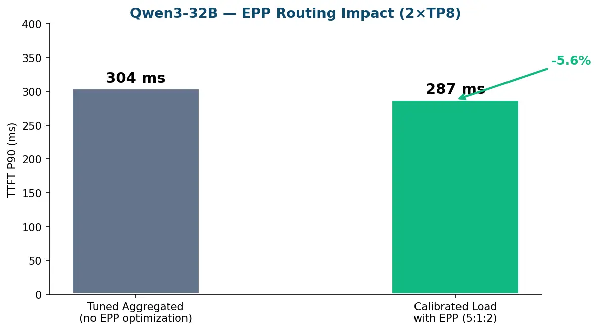
Running at calibrated load (the concurrency level where the system operates at its optimal point rather than full saturation), the cache_optimized EPP routing delivered 287ms TTFT P90 with a P99 of just 611ms. That's compared to 304ms at full 100-user load, a 5.6% improvement from smarter request routing and more appropriate concurrency.
That's a 71% reduction. Same GPUs. Same model. Same workload. Just smarter configuration and smarter routing (figure 3).
Plot twist: Llama-70B
If Qwen3-32B was a satisfying story of improvement, Llama-70B FP8 was a redemption arc. And every good redemption arc starts with things going wrong.
The regression problem
When I upgraded from Red Hat AI Inference 3.3 to 3.4, something interesting happened. The same 2×TP8 configuration that delivered 831ms TTFT in 3.3 now showed 1,292ms in 3.4. Same hardware, same model — different behavior (figure 4).
That's not a bug. Red Hat AI Inference 3.4 introduced prefix-cache-aware routing in EPP, which fundamentally changes how requests flow through the system. The old configuration was tuned for the old routing — it was no longer the right fit.
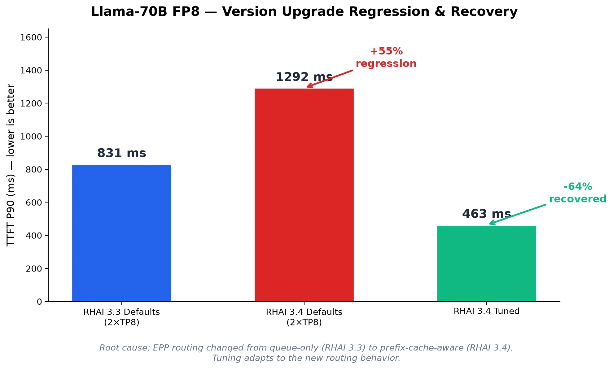
This is actually one of the most important lessons from this experiment: When infrastructure evolves, configuration must evolve with it. The 3.3 defaults were tuned for queue-based routing. The 3.4 stack routes by prefix cache affinity — a smarter strategy that benefits most workloads, but one that needs its own tuning pass. Running 3.4 with a 3.3 configuration is like putting diesel in a car that was just converted to electric.
The baseline
Here are the baseline results.
2x TP8
- Architecture: Aggregated
- TTFT P90: 1,292ms
- Throughput: 27.0 req/s
3P+1D TP4
- Architecture: PD Disaggregated
- TTFT P90: 925ms
- Throughput: 25.6 req/s
Look at that aggregated throughput: 27.0 req/s from 16 H200 GPUs. That's roughly $80 per hour in GPU time, running 24/7 whether your configuration is optimal or not. Your CFO doesn't care that your GPUs are technically capable — they care that the invoice says $58,000 per month. And here's the thing: Lower TTFT isn't just about user experience, it means each request occupies the GPU for less time, which means more requests per second from the same hardware. A 71% TTFT reduction doesn't just make users happier, it means you serve the same traffic with fewer GPUs, or more traffic without buying new ones.
The tuned results
The tuned aggregated configuration achieved 463ms TTFT and 26.9 req/s -- a massive improvement over the default.
2x TP8
- Architecture: Aggregated
- TTFT P90 (ms): 463
- Throughput (req/s): 26.9
- Key Parameters: gmu=0.95, mns=1433, bs=128
3P+1D TP4
- Architecture: PD Disaggregated
- TTFT P90: 681ms
- Throughput: 25.2 req/s
- Key Parameters:
gmu=0.95, mns=1433, bs=128
2x TP8 + EPP
- Architecture: Agg + EPP Tuned
- TTFT P90: 474ms
- Throughput: —
- Key Parameters: EPP weights 4:1:2 (smart-derived)
Not only did I fully recover from the 3.3-to-3.4 regression, I blew past it. The 3.3 baseline was 831ms, and the tuned 3.4 result is 463ms — a 44% improvement over the previous version's best.
max_num_seqs = 1,433?!
The most striking difference between Qwen and Llama tuning is max_num_seqs. At the same TP=8, Qwen gets 192 while Llama gets 1,433. That's a 7.5x difference!
Why? Llama 70B uses grouped-query attention (GQA) with 8 KV heads. This means each sequence's KV cache is relatively compact, so you can fit many more sequences in memory. Meanwhile, Qwen's activation memory profile is the binding constraint. Same formula, wildly different result because of different model architectures.
If I had used Qwen's max_num_seqs=192 for Llama, I would have left 87% of my concurrency capacity unused. If I had used Llama's max_num_seqs=1,433 for Qwen, I would have OOM'd. The lesson: Model-specific tuning is not optional, it's survival (figure 5).
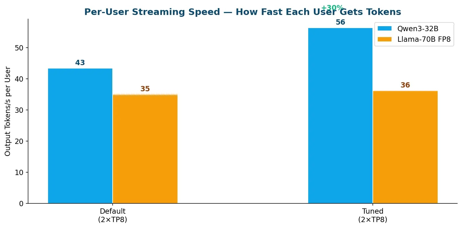
EPP tuning for Llama
For Llama, the smart EPP derivation found a slightly different optimal setting (4:1:2 instead of 5:1:2). The prefix_cache weight dropped by 1 because Llama's larger KV cache per sequence means the kv_cache signal becomes relatively more important. The derivation process detected this automatically from the Prometheus metrics — a genuine case where the smart adjustment improved on the preset.
The regression was fully recovered, and then some: 463ms vs. the original 831ms. That's a 44% improvement over the old version.
What I learned
After dozens of runs across 2 models, 2 architectures, and hundreds of configurations, here are the key takeaways:
Tuning adds 34-56% TTFT improvement beyond version changes
Upgrading from Red Hat AI Inference 3.3 to 3.4 changed performance — sometimes for the better, sometimes not. But in every case, tuning on top of the version upgrade yielded an additional 34-56% TTFT improvement. The version change is table stakes, tuning is where the real gains live.
Optimal configuration shifts between versions
The best config for vLLM 3.3 was not the best config for 3.4 due to different TP degrees, different replica counts, different parameter values. This means tuning is not a one-time activity. Every time you upgrade your inference stack, you need to re-tune.
max_num_seqs formula matters hugely
I cannot stress this enough: max_num_seqs varies enormously between models. Qwen3-32B at TP=8 gets 192, while Llama-70B-FP8 at the same TP=8 gets 1,433. Using the wrong value either wastes GPU capacity (too low) or causes OOM crashes (too high). A multi-factor formula that considers activation memory, KV cache capacity, workload concurrency, and a scheduler cap was one of the most impactful engineering decisions in the entire optimization process.
EPP weights matter for prefix-heavy workloads
For prefix-heavy workloads, the cache_optimized preset (5:1:2) consistently outperformed the upstream default (3:2:2). Smart derivation validated the preset for Qwen and found a minor improvement (4:1:2) for Llama. The lesson: Choosing the right preset matters more than fine-tuning individual weights.
PD consistently beats aggregated for TTFT (but requires RDMA)
In almost every configuration, PD disaggregation delivered lower TTFT than aggregated mode. However, the gap narrows significantly with proper tuning. My tuned aggregated configs came remarkably close to — and in one case beat — untuned PD configs. If you do not have RDMA, don't despair: A well-tuned aggregated deployment can still deliver excellent latency.
Every setup deserves its own configuration
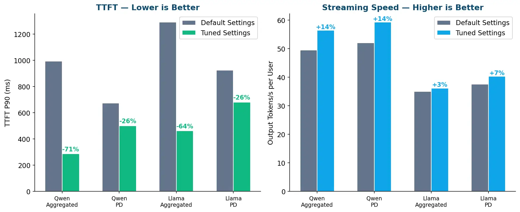
The default templates are designed to be safe and universal — and they do that job well. But every hardware and workload combination has its own sweet spot (figure 6). The difference between generic defaults and hardware-specific tuning was 21-64% TTFT improvement on my setup. Your mileage will vary, but it will almost certainly vary in the right direction.
Summary results
| Model | Stage | Best Config | TTFT P90 | Throughput (req/s) | TTFT Improvement |
|---|---|---|---|---|---|
| Qwen3-32B | 3.4 Default | 8xTP2 (Agg) | 995ms | 24.6 | Baseline |
| 3.4 Tuned | 2xTP8 (Agg) | 304ms | 23.6 | -69% | |
| 3.4 Tuned+EPP | 2xTP8 (Agg) | 287ms | — | -71% | |
| 3.4 Tuned | 6P+2D TP2 (PD) | 501ms | 23.2 | -50% | |
| Llama-70B | 3.4 Default | 2xTP8 (Agg) | 1,292ms | 27.0 | Baseline |
| 3.4 Tuned | 2xTP8 (Agg) | 463ms | 26.9 | -64% | |
| 3.4 Default | 3P+1D TP4 (PD) | 925ms | 25.6 | Baseline (PD) | |
| 3.4 Tuned | 3P+1D TP4 (PD) | 681ms | 25.2 | -26% |
ServeIt Studio for testing
If you've been reading carefully, you might have noticed I tested 95 configurations across 3 architectures. I swept 4 TP values for both decode and prefill. I computed a calibrated load using Little's Law — measuring actual throughput and response time to find the concurrency level that puts the system at its optimal operating point, neither underloaded nor saturated. I derived EPP weights from Prometheus metrics, adjusting each weight based on measured prefix cache hit rates and queue depths. I ran A/B tests with different routing strategies. I computed max_num_seqs from a 4-factor formula involving activation memory, KV cache capacity, workload concurrency, and scheduler caps. I measured block_size impact against prefix cache alignment. I validated everything at calibrated load to confirm sustainable production performance.
Did I do all of this manually? Absolutely not. I would still be running tests.
I built a tool called ServeIt Studio that automates the entire process. It's an automated 12-step inference optimization pipeline that runs on Kubernetes. You point it at your cluster, specify your model and workload, and it handles everything: TP calibration (isolating decode with ISL=1 and prefill with OSL=1), architecture search across aggregated and PD configurations, engine parameter tuning from first principles, EPP weight optimization using measured metrics, and final validation at calibrated load. You come back a few hours later with a fully optimized configuration and a detailed report explaining every decision.
The pipeline starts with infrastructure setup and monitoring, runs decode and prefill TP calibrations, analyzes cluster capacity, generates feasible P/D splits, sweeps aggregated and disaggregated configurations, computes the Pareto front, tunes EPP weights via smart derivation, and finishes with calibrated load validation. Each step builds on the results of the previous steps, narrowing the search space and converging on the optimal configuration. I'll cover the tool's architecture and the 12-step pipeline in detail in a future article.
The point of this post is not the tool, though, it's the results. Whether you tune manually or use automation, these optimizations are real, measurable, and available to anyone running vLLM on Kubernetes.
Conclusion
I started with 995ms TTFT. I ended with 287ms TTFT. Same GPUs, same model, same workload. The only difference was configuration — 71% better latency.
Your GPUs are not slow. They just have not been introduced to their full potential yet. The default settings keep everything running safely, but matching the configuration to your specific hardware and workload is where the real performance lives.
The only question is whether you want to spend weeks doing it by hand, or let a tool do it in hours. ServeIt Studio is open source and available at github.com/openshift-psap/serveit-studio.