In the previous post in this series, we built a streaming retrieval-augmented generation (RAG) pipeline that parses, chunks, embeds, and writes to Milvus in a single Ray Data script. It works well. But it is a monolithic script. When parsing fails at file 847 of 1,000, you rerun everything from scratch. When someone asks what parameters produced last Tuesday's vector collection, you search through logs using grep. When you want to swap the embedding model, you edit the same file that owns the parser, the chunker, and the Milvus writer.
If you are an MLOps engineer or AI practitioner looking to move from experimental scripts to production RAG orchestration, this guide demonstrates how to deploy modular, maintainable workflows on OpenShift AI.
This is the 4th post in our series on scaling RAG document processing. The 1st post made the business case for distributed processing. The 2nd post showed how to scale Docling parsing on Red Hat OpenShift AI. The 3rd post unified parsing, embedding, and vector storage into a single streaming job.
This post wraps the same Ray Data and Docling processing in AI pipelines, giving you reproducible parameterized runs with full history, S3-compatible intermediate storage that enables independent component retries, and 5 reusable components you can swap, schedule, or extend individually. The previous post covers the engine; this post adds the production automation layer.
What the RAG pipeline does
The pipeline takes a collection of PDF documents and produces a queryable RAG system with a deployed large language model (LLM). It handles every step: parsing PDFs into structured content, splitting that content into chunks that respect document structure, generating vector embeddings, storing those embeddings in Milvus, and deploying both an embedding model and an LLM for inference.
To move from raw PDFs to a queryable production system, the pipeline combines specialized open source tools within a unified architecture: Docling for structure-aware parsing and chunking, Ray via KubeRay for distributed compute, Milvus for vector storage, MinIO for S3-compatible intermediate storage, and vLLM via KServe for LLM and embedding model serving (using Mistral-7B-Instruct-v0.3 as the default LLM). All orchestrated through Kubeflow Pipelines (KFP) via AI pipelines on OpenShift AI.
Red Hat OpenShift AI is what ties these components into a managed platform rather than a collection of tools you wire together yourself. It handles Ray cluster lifecycle through KubeRay, GPU scheduling and fair sharing through Kueue, model serving with autoscaling through KServe, and self-service pipeline orchestration through AI pipelines—so you focus on the RAG logic, not the infrastructure. For a deeper look at the full technology stack, see the previous post in this series.
Why orchestrate your RAG pipeline with AI pipelines
The streaming pipeline in the previous post is a valid approach for many workloads. But as your RAG system moves toward production, you need capabilities that a single script cannot provide on its own.
Reproducibility and run history
Every pipeline run in AI pipelines records its parameters, timestamps, logs, and status. When a colleague asks what embedding model and chunk size produced the collection running in production, you open the OpenShift AI dashboard and read it directly from the run record. You do not reconstruct it from shell history or environment variables. You can also schedule recurring runs to reingest documents on a weekly cadence, or trigger a run automatically when new documents land in your source bucket.
S3 intermediate storage enables independent retries
We designed this pipeline to write parsed and chunked output as JSONL files to S3 between the parsing and ingestion stages. This is a design choice we made for this pipeline, not a built-in platform feature. The benefit is concrete: if the Milvus ingestion step fails after parsing 1,000 documents, the parsed chunks are already sitting in S3. You fix the Milvus connection and rerun only the ingestion component. KFP supports component-level re-execution, and because the intermediate data lives in S3, the rerun picks up right where the failure occurred without repeating hours of document processing.
Parallel execution chains
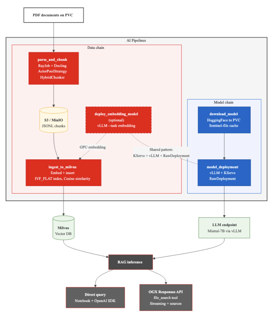
The pipeline runs 2 independent chains concurrently. The data chain handles parsing, embedding, and ingestion. The model chain downloads and deploys the LLM. These chains have no dependency on each other until query time, so running them in parallel cuts total pipeline execution time significantly. A model download that takes 15 minutes happens at the same time as document parsing that takes 20 minutes, rather than running sequentially for 35 minutes total.
Reusable components
Each of the 5 components is a self-contained KFP component with its own container image, parameters, and interface. You can reuse the model deployment component in a completely different pipeline. You can replace the parsing component with one that handles a different document format. The components are building blocks, not a monolith.
The 5 RAG pipeline components
parse_and_chunk
The parse_and_chunk stage submits a RayJob that distributes Docling processing across Ray workers using map_batches with ActorPoolStrategy. Each actor runs Docling's DocumentConverter in a separate subprocess for crash isolation, so a malformed PDF that causes a segfault does not take down the entire Ray worker. The component uses Docling's HybridChunker, which respects document structure when determining chunk boundaries rather than splitting at arbitrary character counts. Output is written as JSONL files to S3, where each line contains the chunk text, source document metadata, and positional information.
ingest_to_milvus
To handle vector indexing, ingest_to_milvus reads the JSONL chunks from S3, generates vector embeddings, and inserts them into Milvus with an IVF_FLAT index configured for COSINE similarity. It supports 2 embedding modes. For collections up to roughly 10,000 chunks, local CPU embedding with the granite-embedding-125m-english model (approximately 500 MB) requires no GPU resources and adds no additional infrastructure. For larger collections exceeding 100,000 chunks, offloading embedding generation to a vLLM service on a dedicated GPU node increases throughput up to 10 times compared to standard CPU workers.
deploy_embedding_model
When enabled, the optional deploy_embedding_model component deploys a text embedding model as a KServe InferenceService using vLLM with the --task embedding flag. It only runs when the pipeline parameter deploy_embedding is set to True. For smaller workloads where local CPU embedding is sufficient, you skip this component entirely and save the GPU resources for model serving. This conditional execution is one of the benefits of the component-based design: the pipeline adapts to your scale without code changes.
download_model
The download_model stage pulls a Hugging Face model to a persistent volume claim (PVC) with sentinel file caching. The first download of a model like Mistral-7B pulls approximately 14 GB of weights, which takes 10 to 20 minutes. On subsequent runs, the sentinel file signals that the model is already present, and the component completes in seconds. This avoids redownloading the model every time a pod restarts or a new pipeline run begins.
model_deployment
Finally, model_deployment provisions the LLM as a KServe InferenceService running vLLM. It follows OpenShift AI dashboard conventions for resource naming and labeling, and integrates with HardwareProfile for GPU allocation. The deployment uses RawDeployment mode, which gives you direct control over the serving configuration without the additional abstraction layers of serverless mode.
Multi-step RAG pipeline architecture
The multi-step pipeline, separates the data processing into 3 sequential components (parse_and_chunk, optionally deploy_embedding_model, then ingest_to_milvus) and runs 2 model components (download_model, then model_deployment) in parallel. You can inspect the complete component definition in the OpenDataHub GitHub repository. This production-oriented variant gives you independent component retries, clearer failure isolation, and the ability to rerun only the stages that need updating.
Running the RAG pipeline
Prerequisites
You need:
- An OpenShift AI cluster with AI pipelines enabled
- KubeRay operator installed
- Milvus and S3-compatible storage deployed
- A Hugging Face token with access to the LLM you plan to deploy
- GPU nodes for model serving
- A workbench with the pipeline SDK installed
Getting started
The example repository includes a guided notebook, rag_pipeline_build.ipynb, that walks you through configuring parameters, compiling the pipeline, and submitting it to AI pipelines. The notebook handles S3 credentials, Milvus connection details, model selection, and worker scaling configuration. You can choose between the single-step and multi-step variants depending on whether you are in development or production mode.
Once the pipeline completes, the repository includes 2 options for querying the deployed RAG system. The rag_query_test.ipynb notebook lets you validate the end-to-end system by submitting queries directly against the deployed LLM with Milvus-backed retrieval, giving you full control over retrieval parameters like top-k and similarity thresholds.
For a more integrated approach, the rag_ogx_streaming.ipynb notebook demonstrates querying through the OpenGenAI Stack (OGX) Responses API, which is included with Red Hat OpenShift AI. A single API call with the file_search tool handles the entire retrieval-augmented generation flow—vector search, context retrieval, grounded generation, and streaming—with built-in source attribution. This collapses the manual embed-search-prompt-generate loop into 1 request.
How this fits the series
This series has progressively built up the production RAG architecture. The 1st post explained why distributed processing matters. The 2nd post focused on scaling Docling parsing alone. The 3rd unified parsing, embedding, and ingestion into a single streaming pipeline. This post adds the orchestration layer that makes the whole system reproducible, observable, and maintainable in production. Each post builds on the one before it, and each addresses a different layer of the problem.
Get started
Clone the example repository and follow the guided notebook to deploy the full pipeline on your OpenShift AI cluster. Once you run through the notebook, you will have a reproducible, multi-step RAG pipeline processing your own documents on OpenShift AI. The README file walks you through every prerequisite and configuration step.
Try running the pipeline with your own document sets or adapting the components to your existing storage layers. Have questions or custom components to share? Open an issue or start a discussion in the Red Hat AI examples repository.
To learn more about the platform, explore the Red Hat OpenShift AI documentation and AI pipelines documentation.
Series note
Explore the full RAG scaling series: