When building fraud detection systems, standard training steps often hide expensive failures. A model can show 96% accuracy on paper while letting every single fraudulent transaction pass unchecked. In fraud detection, a common first pass uses logistic regression with basic features and a 0.5 threshold. which often yields an accuracy of 96%. That yields 96% accuracy because 96% of the transactions are legitimate—meaning a model labeling everything as legitimate gets 96% of its calls right while catching zero fraud. This is why accuracy is the wrong metric: it measures how well the model handles the majority class rather than exposing failure. A better metric is recall, which measures the share of fraud actually caught.
The defaults drift toward this exact failure: without class weighting, the model treats every row equally during training, so fraud's 4% share pulls its predicted probabilities well below a 0.5 threshold, and it barely flags anything.
The way out is searching the model space and scoring candidates on a metric the failure can't hide behind. This demo does exactly that. In this post, we will walk through a local Python pattern for cost-ranked model selection first, and then show how to scale the same workflow using Red Hat OpenShift AI. The demo sweeps a space of model configurations against held-out data, finds the classifier you'd miss by shipping the defaults, and hands the winner's output to a large language model (LLM), which drafts the note a fraud analyst reads. The search here is hand-built in Python rather than run through the automated machine learning (AutoML) feature in Red Hat OpenShift AI, and the metric it ranks by is a custom cost function. Both choices are deliberate because they keep the underlying code and custom scoring logic explicit.
The loop
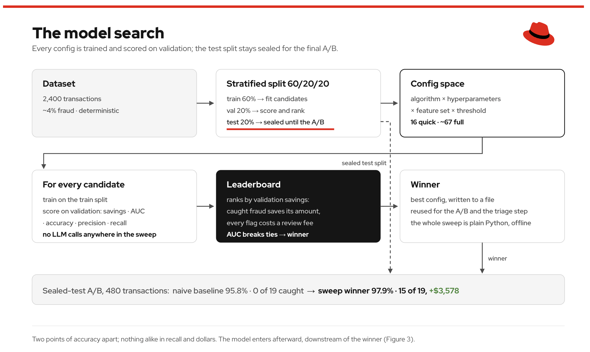
Instead of manually tuning a single configuration, you can run a systematic sweep across model variations and let held-out validation data prove which candidate wins. Concretely, that means defining a search space, training every candidate in it, evaluating each on data the training never saw, and keeping whichever ranks best. Here, the space has 5 dimensions: algorithm choice, hyperparameters, feature set, extra training weight for fraud rows, and the decision threshold.
The real design question is what to rank the candidates by. Accuracy can't do it for the reason explained above; with imbalanced data, nearly every candidate lands in the mid-90s. Recall alone breaks in a different way: a model that flags every single transaction catches all fraud, but floods the review queue with false positives.
So, the leaderboard ranks candidates by a custom cost metric instead. Every fraudulent transaction the model catches counts as money saved (the transaction amount). For this model, we assign an estimated cost of US$6 per flagged transaction to account for human analyst review time. Adding those up gives each candidate 1 number pricing both mistakes: missed fraud and false alarms. Rhis cost function is tailored specifically for this demonstration workflow.
The sweep
The dataset used in the demo contains 2,400 generated transactions, with about 4% of them being fraudulent. Because the generator is deterministic, every run reproduces the same data. Its fraud patterns are deliberately hard to spot—for example, card-not-present sprees, late-night gift card runs, foreign-country transactions, and activity engineered to look like ordinary spending. From there, the data splits 60/20/20 into train, validation, and test sets, stratified so each split maintains that same 4% rate. The sweep never touches the test split, which stays sealed until the final comparison.
That 4% rate and those overlapping patterns are design choices, and the dollar figures follow from them. The dataset is synthetic, so read the numbers as a demonstration of the problem rather than a precise measurement. None of that changes the ordering. Once fraud is rare enough that nearly every candidate lands in the mid-90s, accuracy stops separating them, and whatever you rank by instead decides which model ships.
To balance execution speed with thoroughness, the search scales from a rapid 16-configuration sanity check to a full 67-model sweep across 3 algorithm families (logistic regression, decision trees, and random forests) across small hyperparameter grids, 3 feature sets, and a range of thresholds. The sweep scores each candidate on the validation split using 3 metrics:
- Estimated cost impact: Every caught fraud saves its transaction amount, and every flag costs a fixed US$6 analyst review fee.
- Area Under the ROC Curve (AUC): Measures how consistently a model distinguishes between real transactions and fraud from non-fraud across different sensitivity levels, serving as the tiebreaker between candidates with similar cost impact.
- Accuracy, precision, and recall: Printed alongside, these metrics show how little accuracy separates the candidates.
Logistic regression still won with the baseline's 0.5 threshold, but it won on feature set and class weight instead. It used all 12 columns (up from 3), including behavioral features, and counted fraudulent rows 4 times heavier during training. That weighting corrects for a skewed class without resampling the data, which a default first pass never does.
Then comes the A/B test on the untouched test split. The naive baseline scores 95.8% accuracy and catches 0 of 19 test frauds. The winner scores 97.9% and catches 15 of 19, coming out about US$3,578 ahead of the baseline in net savings over the 480 test transactions.
That's 2 percentage points of accuracy between a model that misses almost everything and one that catches most of it. If accuracy were the only number on the screen, they'd look nearly interchangeable.
Where the LLM enters
The LLM enters after the classifier has decided, not before. For a transaction the winner flags, the demo collects the risk score and the evidence behind it. The values influencing these scores include the amount ratio against the customer's normal spending, the card-present flag, the hour, and the country. Those facts go into the LLM prompt, and the LLM drafts the analyst note. Run the same transaction under the baseline config and it scores below the threshold, so no note is ever written. The analyst never sees it because the model never flagged it.
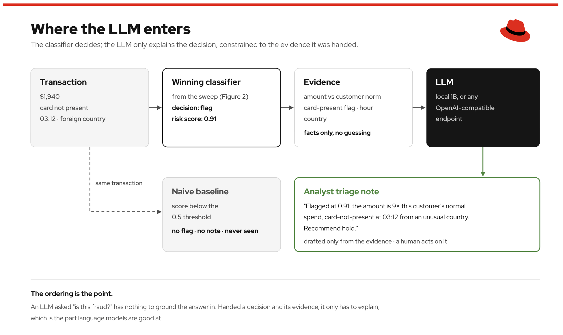
Figure 2: The classifier decides and supplies the evidence; the LLM drafts the note from that evidence, and a human acts on it.
The ordering matters because asking an LLM "Is this fraud?" directly with nothing to ground the answer in is a recipe for hallucination. But when handed a decision and its underlying evidence, asking the LLM only to explain relies on concrete inputs, which matches what language models do best. This pattern wasn't invented just for this demo. The AutoML announcement calls combining predictive AI outputs with gen AI capabilities an emerging pattern. Its example uses the same structure: a predictive model flags an item, and a readable recommendation reaches a human.
The demo versus the platform feature
Everything above is the core idea, kept small. The AutoML feature in Red Hat OpenShift AI (currently in Technology Preview) runs a much bigger version of the same loop. Its optimization is an AI pipeline built on Kubeflow Pipelines and the open source AutoGluon library. AutoGluon searches and ensembles far more model families than the demo's 3, uses staged fitting strategies rather than an exhaustive grid, and covers binary and multiclass classification, regression, and time-series tasks. Its leaderboard lives in the dashboard, where you can open an interactive notebook for the best model or register it for deployment.
The division of labor is different, though. AutoML selects the algorithms, hyperparameters, data split, and evaluation metric itself, automating most setup this demo performs by hand. For binary classification, it optimizes accuracy, so you'd apply a cost calculation like this custom metric to the leaderboard after the run finishes.
Sweep locally, scale with OpenShift AI model serving
The demo runs entirely on a laptop. The sweep uses standard-library Python and stays offline, while the LLM step uses a local 1-billion-parameter model through Ollama (or any OpenAI-compatible endpoint if you switch the backend). Run it from the repository and you also get a web app in your browser containing the leaderboard, the baseline-versus-winner A/B test on the test split, and a triage tab handing the winner's evidence to the model.
Moving this workflow from a laptop to Red Hat OpenShift AI requires swapping local components for enterprise platform services:
- A local CSV file moves to object storage in Amazon S3, integrated directly into OpenShift AI.
- A hand-built Python grid search becomes an AutoML optimization run using AutoGluon on Kubeflow Pipelines, with the search space, algorithms, and evaluation metric selected for you.
- The printed leaderboard becomes the AutoML leaderboard in the dashboard, complete with sortable metrics, a confusion matrix, and feature importance.
- The winning configuration becomes a model registered to the model registry and served from a REST endpoint.
- A local 1-billion-parameter model writing the triage note becomes an LLM served by vLLM—a separate serving capability that your application calls, not part of the AutoML feature itself.
The production side of each swap is Red Hat OpenShift AI, where AutoML is a Technology Preview alongside AutoRAG.
The takeaway
On imbalanced data, the default workflow can fail without leaving a trace in the accuracy number; in this demo, it reported 96% while missing fraud almost entirely. The same trap appears anywhere the positive class is rare, such as medical screening, network intrusion, or manufacturing defects. In none of those scenarios is rarity a data collection problem fixed by sourcing a more balanced dataset. It's the shape of the problem, so the model must be evaluated against that shape: validation data representing the distribution it will actually run in, and a ranking metric pricing what a mistake costs in that distribution. Accuracy does neither. A cost-based metric, like the custom calculation in this demo, does both.
The way out is searching the space instead of shipping defaults and ranking on a metric that reflects the model's purpose. Then keep the LLM downstream of the decision, turning the winner's evidence into a note a human can act on rather than a raw probability. Run the sweep on the committed dataset and check where the baseline lands on the leaderboard.
Explore the full code, run the sweep on your machine, and experiment with custom cost functions in the GitHub repository.
Resources
- Access the fraud model search demo on GitHub (located in the
automl/directory) - Explore AutoML and AutoRAG in Red Hat OpenShift AI