There is a major push in the United Kingdom to replace aging mechanical electricity meters with connected smart meters. New meters allow consumers to more closely monitor their energy usage and associated cost, and they enable the suppliers to automate the billing process because the meters automatically report fine-grained energy use.
This post describes an architecture for processing a stream of meter readings using Strimzi, which offers support for running Apache Kafka in a container environment (Red Hat OpenShift). The data has been made available through a UK research project that collected data from energy producers, distributors, and consumers from 2011 to 2014. The TC1a dataset used here contains data from 8,000 domestic customers on half-hour intervals in the following form:
 Location ID,Measurement Description,Parameter Type and Units,of capture,Parameter
 120,Electricity supply meter,Consumption in period [kWh],03/12/2011 00:00:00,0.067
 120,Electricity supply meter,Consumption in period [kWh],03/12/2011 00:30:00,0.067
 120,Electricity supply meter,Consumption in period [kWh],03/12/2011 01:00:00,0.066
 120,Electricity supply meter,Consumption in period [kWh],03/12/2011 01:30:00,0.066
As a single year of data represents approximately 25GB of comma-separated value (CSV) data, so importing and analyzing this data on a single machine is challenging. Also, when considering the relatively small number of customers monitored (8,000) in comparison with the number of actual customers served by any reasonably sized power company, the difficulties in processing this stream of data are magnified.
The approach adopted here is to process this data in the form of a stream of readings and make use of the Red Hat AMQ Streams distributed streaming platform to perform aggregations in real time as data is ingested into the application. The outputs of the system will be twofold: a dataset that can be used to train models of consumer use over a 24-hour period and a monitoring dashboard showing live demand levels.
Components
In order to architect a system that could scale to be deployed in a production environment, we adopted a microservices approach deployed on Red Hat OpenShift. The microservices are connected via Apache Kafka topics in the following pipeline:
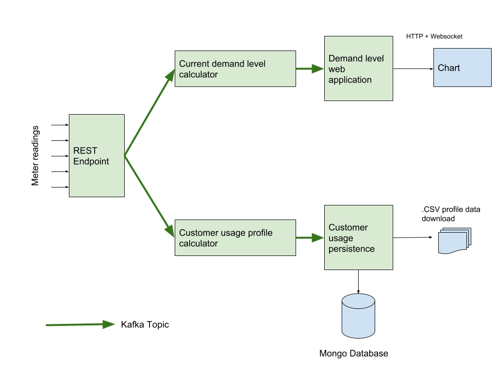
Each of these blocks is deployed individually within OpenShift and makes use of an Apache Kafka Cluster provided by AMQ Streams.
The CloudEvents specification aims to enable portability of applications across multiple cloud providers. This is an ideal fit for describing the meter reading values that are sent from smart meters (or a simulator, in our case) to the energy supplier. Such portability will enable customers to change their electricity supplier without needing to change the hardware in their homes.
REST Endpoint
Data is ingested into the system via a Smart-Meter Simulator (which just reads the CSV data file) on a reading-by-reading basis. These meter readings are sent as CloudEvents to a RESTEasy microservice running as a Thorntail application. The application is deployed to OpenShift using the Fabric8 Maven plugin and converts the CloudEvents into Apache Kafka messages stored by AMQ Streams. This microservice makes use of the Kafka CDI library, which enables interaction with Apache Kafka topics via simple CDI annotations within Java code. This means that to connect to an Apache Kafka topic and send data to it, the amount of code is dramatically reduced to this:
@ApplicationScoped
@Path("/clnr")
@KafkaConfig(bootstrapServers = "#{KAFKA_SERVICE_HOST}:#{KAFKA_SERVICE_PORT}")
public class IngestAPI {
private static final SimpleDateFormat format = new SimpleDateFormat("yyyy/MM/dd HH:mm:ss");
private final static Logger logger = Logger.getLogger(IngestAPI.class.getName());
@Producer
private SimpleKafkaProducer<String, Reading> myproducer;
The @KafkaConfig annotation defines the location of the Apache Kafka cluster that will be used. This configuration can be entered directly or, if the data is formatted as #{VALUE}, it will be taken from environment variables. This is useful when deploying the service into OpenShift as environment variables that are a key route for adding configuration data to deployments. The @Producer annotation defines an output to an Apache Kafka topic where the code can send messages. Changes to the application configuration are handled transparently by OpenShift; a container is restarted if its configuration changes.
As part of any stream processing application, the correct consideration of timestamps within the data is essential. By default, the Apache Kafka Streams API adopts the system time (that is, wall clock time) when processing messages. So, if a message has been placed onto a topic without a timestamp in place, the default behavior will be to add a timestamp representing the current instance in time. Given that the data we are processing has been generated by other systems at a prior time to it being received, we need to configure Apache Kafka to use a timestamp that is embedded in the message payload.
There are two ways of achieving this:
- Tell Apache Kafka to use a timestamp extractor class to explicitly pull a timestamp from the messages. Apache Kafka provides a mechanism for doing this when attaching the Streams API to a topic.
- Add a timestamp to a message before it is placed onto a topic. This is the approach adopted in this example, primarily because the Kafka CDI library does not yet support the declaration of a timestamp extractor class in the streams annotation.
To include a timestamp in a message, a new ProducerRecord object must be created with the required metadata:
Long timetamp = reading.getReadingTime();
String key = reading.getCustomerId();

ProducerRecord<String, Reading>; record = new ProducerRecord<>(“readings”, null, timestamp, key, reading);

((org.apache.kafka.clients.producer.Producer)myproducer).send(record);
Here are some points to consider:
- The timestamp and key are obtained directly from the parsed meter reading created when a row of data is posted into the ingest API.
- It is necessary to explicitly cast the
SimpleKafkaProducerinjected by the Kafka CDI library into an Apache KafkaProducerobject in order to be able to send aProducerRecorddirectly. When the Kafka CDI library is extended to include a timestamp extractor class annotation, this code to directly insert a timestamp would no longer be necessary.
Current Demand-Level Calculator
The purpose of the demand-level aggregator is to collect all of the readings in a one-hour period for all of the consumers in the dataset in order to provide an hour-by-hour demand level. In order to do this using the Apache Kafka Streams API, we need to aggregate the data into a rolling one-hour window. The code for this is shown below:
@KafkaStream(input="ingest.api.out", output="demand.out")
    public KStream<String, JsonObject> demandStream(final KStream<String, JsonObject> source) {
        return source
                /*.peek((k, v)->v.toString())*/
                .selectKey((key, value) -> {
                    return "ALL";
                }).map((key, value) -> {
                   MeterReading mr = new MeterReading();
                   mr.setCustomerId(value.getString("customerId"));
                   mr.setTimestamp(value.getString("timestamp"));
                   mr.setValue(value.getJsonNumber("kWh").doubleValue());
                   return new KeyValue<>(key, mr);
               })
                .groupByKey(Serialized.with(new Serdes.StringSerde(), CafdiSerdes.Generic(MeterReading.class)))
                .windowedBy(TimeWindows.of(1 * 60 * 60 * 1000).until(1 * 60 * 60 * 1000))
                .aggregate(() -> 0.0, (k, v, a) -> a + v.value,
                        Materialized.<String, Double, WindowStore<Bytes, byte[]>>as("demand-store")
                                .withValueSerde(Serdes.Double())
                                .withKeySerde(Serdes.String()))
                .toStream().map(new KeyValueMapper<Windowed<String>, Double, KeyValue<String, JsonObject>>() {
                    @Override
                    public KeyValue<String, JsonObject> apply(Windowed<String> key, Double value) {

                        JsonObjectBuilder builder = Json.createObjectBuilder();
                        builder.add("timedate", format.format(new Date(key.window().start())))
                                .add("hour", hourFormat.format(new Date(key.window().start())))
                                .add("day", dayFormat.format(new Date(key.window().start())))
                                .add("timestamp", key.window().start())
                                .add("demand", value);

                        return new KeyValue<>("DEMAND", builder.build());
                    }
                }
           )
In this code, there are a number of distinct steps to perform:
.selectKey((key, value)
When the data is ingested, the data in the input stream is keyed by customer ID; however, in this aggregation we want to group data from all users into a single set of time windows that represent the usage data for a particular hour. In order to do this, we apply a selectKey operator that simply replaces the customerId field with a default key of “ALL”.
map((key, value)
The data passed between the various steps in this prototype is formatted as plain JSON as a lowest-common-denominator format. We are going to treat the data as a stream of MeterReading objects, so this map operator parses each record in the stream in turn and returns instances of the MeterReading Java object.
groupByKey
To perform any windowing operators, the Apache Kafka Streams API requires us to group the incoming data into a KGroupedStream. Because we have already replaced the customerId field with a standard key, this operator produces a grouped stream with a single group within it.
.windowedBy(TimeWindows.of(1*60*60*1000).until(1*60*60*1000))
This is the operation that collects data from the input stream of meter readings into one-hour long windows of readings. In order to cater to some out-of-order events such as delayed readings, we retain this window of data for one hour after its time span. This allows us to insert events into this window up to one hour after they were expected to arrive. This parameter is clearly tunable and in a real system would be adjusted to balance between having results produced in an acceptable time span and potentially ignoring data that arrives too late.
.aggregate(() ->0.0, (k, v, a) -> a + v.value
This step performs the actual work of adding up all of the meter readings in a single time window. The values are summed using an aggregator, which is initialized as a double-precision value of 0.0 and, when new readings fall within the window, this value is updated with the current meter reading value.
public KeyValue<String,JsonObject> apply(Windowed<String>key,Double value)
Once we have a stream of total values for each time window, we apply another mapping function to these to add extra data such as timestamps, hour of data, and so on. This stream is then passed on to the downstream topics as JSON objects.
Demand-Level Web Application
Once a stream of hourly total demand level has been produced, the next step in the pipeline is to display this data via a simple visualization. Because the nature of this prototype is to investigate the feasibility of using Apache Kafka streams to process smart-meter data, the visualization in this demo is extremely simple in nature and just displays a bar chart that is updated when new hourly demand levels are available.

In addition to the web chart, two other components are present in this application:
Kafka CDI Topic Connection
This component uses the simplest form of the Kafka CDI library to create a consumer method that receives demand-level JSON objects from the output of the demand-level calculator application:
@ApplicationScoped
@KafkaConfig(bootstrapServers = "#{KAFKA_SERVICE_HOST}:#{KAFKA_SERVICE_PORT}")
public class DemandStreamListener {

    public DemandStreamListener() {
        System.out.println("Started demand stream listener");
    }

    private static final Logger logger = Logger.getLogger(DemandStreamListener.class.getName());

    @Consumer(topics = "demand.out", groupId = "1")
    public void onMessage(String key, JsonObject json){
        logger.info(json.toString());
        DemandWS.sendDemand(json);
    }
The key part of this code is the @Consumer annotation, which attaches to the Apache Kafka topic and marks the onMessage method as the receiver for JsonObject messages from the demand.out Apache Kafka topic. As soon as messages are received, they are simply passed directly to the DemandWS websocket.
Websocket Handling
In order to pass messages directly to the browser to support dynamic chart updating, we create a simple WebSocket endpoint that just keeps a list of connected WebSockets and passes demand level messages to each, in turn, every time a new message is received from the Kafka topic:
@ServerEndpoint("/ws")
@ApplicationScoped
public class DemandWS {
    private static final Logger logger = Logger.getLogger(DemandWS.class.getName());

    public static final Map<String, Session> clients = new ConcurrentHashMap<>();

    @OnOpen
    public void socketOpened(Session client){
        logger.info("Socked Opened: " + client.getId());
        clients.put(client.getId(), client);
    }

    @OnClose
    public void socketClosed(Session client){
        logger.info("Socket Closed: " + client.getId());
        clients.remove(client.getId());
    }

    public static void sendDemand(JsonObject demandMessage){
        for(Session client : clients.values()){
            client.getAsyncRemote().sendText(demandMessage.toString());
        }
    }
}
The WebSocket implementation is extremely simple: it uses the @ServiveEndpoint annotation to mark it as a WebSocket endpoint. This then allows clients to connect and receive real-time updates. The implementation tracks the lifecycle of the client connections so that messages can be routed to the currently active clients when new demand-level Apache Kafka messages are received.
Customer Profile Aggregator
The aim of the Customer Profile Aggregator microservice is to construct average usage patterns across the day for each customer. This is divided into 24-hour values representing the average amount of energy that a customer uses in that hour. These values can be combined with other datasets and used in machine learning applications, for example, to predict social class or future usage patterns for capacity planning.
As with the microservice that calculates the current demand, the profile aggregator makes use of the Apache Kafka Streams API to process the data.
source.selectKey((key, value) -> value.getString("customerId"))
       .groupByKey(Serialized.with(new Serdes.StringSerde(), new MeterReadingSerializer()))
       .aggregate(()->new CustomerRecord(), (k, v, a)-> a.update(v), CafdiSerdes.Generic(CustomerRecord.class))
       .toStream().map((k, v)->{
           String json = "";
           try {
               json = mapper.writeValueAsString(v);
           } catch (Exception e){
               e.printStackTrace();
           }
           return new KeyValue<>(v.customerId, json);
       });
Processing the data using the Apache Kafka Streams API is straightforward. Initially, records are grouped by the ID of the customer they relate to. Following this, they are converted to a CustomerRecord object. This object contains a bucket for each hour of the day holding the energy used in that hour. When the CustomerRecord for each customer is updated with a new MeterReading, the relevant bucket is updated. Finally, the output is written as a JSON-formatted stream of CustomerRecords. These records are persisted to a database to allow them to be consumed by other applications that are not necessarily developed in a streaming-aware manner.
There is a download REST service that can query this database to give the current hourly usage profiles of all of the customers in the form of a CSV file that can be imported into spreadsheets for analysis or used for machine learning and customer classification.
Packaging the Components
Because we are running this stack within OpenShift and making use of the AMQ Streams–packaged Apache Kafka platform, there are some considerations to be made when packaging and deploying the various components. Where applicable, the components are packaged as microservices using WildFly Swarm with the microprofile features enabled. This is reflected in the pom.xml dependencies on org.wildfly.swarm:microprofile and org.aerogear.kafka:kafka-cdi-extensions.
These dependencies are sufficient to enable the CDI environment that manages the injection of Apache Kafka connections which are used to transport messages. One thing that this does not provide yet, however, is the deployment and management of the requisite Apache Kafka topics which need to be present for the Kafka CDI injection process to work. Fortunately, AMQ Streams provides a route for declaratively creating Apache Kafka topics via config maps, which are an OpenShift/Kubernetes mechanism for providing key:value configuration properties to deployed applications.
To create a new topic, the following ConfigMap entries need to be created:
apiVersion: v1
kind: ConfigMap
metadata:
  name: demand.out
  labels:
    strimzi.io/kind: topic
    strimzi.io/cluster: my-cluster
data:
  name: demand.out
  partitions: "2"
  replicas: "1"
The critical sections of this map lie in the labels attributes. The AMQ Streams operator continuously monitors the config maps within the environment, and when maps containing the strimzi.io labels appear, the operator will take steps to manage any required Apache KSt topics. The data section in the config map contains the actual details of the topics to be deployed.
Config maps like this are packaged as YAML files and deployed as part of the application using the Fabric8 Maven plugin. The Fabric8 plugin aims to simplify the deployment of microservices in both Kubernetes and OpenShift container environments and provides facilities for packaging up code and configuration into a single deployable unit. By convention, we packaged up the parts of this demo along with configurations for the output topics for each component. By doing this, once all components were deployed, we were left with a fully connected set of deployments exchanging Apache Kafka messages via topics to process the smart-meter data in real time as it was posted to the ingest API endpoint.
Conclusions
Apache Kafka and the Streams API make it fairly easy to perform the kinds of real-time aggregations needed to process this type of data stream. The operators provided for windowing and grouping coupled with the opportunities to add custom aggregators, mapping functions, and so on make for a rich set of stream-processing capabilities.
The Strimzi distribution of Apache Kafka makes it straightforward to deploy a tested, performant Apache Kafka cluster within a container environment with very little configuration effort. This allowed us to focus on the actual stream operators required to process the data
Running the demo in OpenShift provided an environment that allowed us to scale the various parts of the infrastructure to deal with increased volumes of meter readings. By keying the raw reading stream by customer ID we could, if needed, scale the aggregation of individual customer profiles over multiple calculation nodes.
The complex task of deploying all of the various components was greatly simplified through the use of the Fabric8 Maven plugin, which allowed us to package up code, configuration, and Apache Kafka topic definitions into deployable units and deploy these directly into OpenShift with a single command.
Last updated: September 3, 2019