Evaluate AI agents with IBM CLEAR & EvalHub on OpenShift AI

Adopting eval-driven development is essential for building reliable AI agents, but doing it effectively is harder than it looks. Even when your agent handles the basic scenario well, subtle failures surface in production—misusing a tool, going off-topic during a logic step, or returning answers that sound plausible but are incorrect. These are failures unit tests don't catch and logs can't fully explain.

Static benchmarks measure a model's knowledge in isolation. While useful, they leave blind spots regarding how an agent behaves across a multistep workflow, whether tool calls are well-formed, whether retrieval surfaces relevant context, or whether the reasoning chain holds up under real inputs. A core requirement of eval-driven development is trace evaluation: automating the analysis for each step in your agent's execution to surface recurring failure patterns, their frequency, their severity, and where they originate.

This tutorial walks through a complete pipeline on Red Hat OpenShift AI 3.4+:

• MLflow: Captures your agent's execution as structured traces—every LLM call, tool invocation, and node transition—with inputs and outputs preserved.
• IBM CLEAR (Comprehensive LLM Error Analysis and Reporting): A tool for systematic error analysis of agentic systems, using an LLM-as-a-judge approach. For every interaction, it scores reasoning quality, relevance, and tool usage, and generates a short critique, then clusters those critiques into a ranked list of recurring failure patterns, each with a frequency, severity, and attribution to the step or agent where it occurs. So instead of a single aggregate number, you get a view of which systematic issues to fix.
• EvalHub: A framework-agnostic AI evaluation and orchestration service introduced in Red Hat AI 3.4 and integrated with Red Hat OpenShift AI that orchestrates the evaluation as an OpenShift job, accepting submissions via API, routing traces to CLEAR, and storing results back in MLflow.

We run the evaluation in 2 modes:

• Standard mode (separate_tools: false): Evaluates each agent step holistically, including any tool calls made within the step.
• SPARC (Semantic Pre-execution Analysis for Reliable Calls) mode (separate_tools: true): Separates tool calls into their own scoring rows, giving finer-grained analysis of tool usage correctness versus reasoning quality.

By the end of this guide, you will have an automated evaluation pipeline that surfaces recurring agent failures, saving your engineering team from hours of manual log inspection..

Prerequisites

• Red Hat OpenShift AI 3.4 or later cluster with admin access
• oc CLI configured and authenticated (oc whoami succeeds)
• Python 3.11 or later with either the EvalHub software development kit (SDK) or MLflow installed (for uploading traces):

pip install "eval-hub-sdk[adapter]"

• An OpenAI-compatible judge LLM endpoint: Any model that exposes a /v1/chat/completions API works. This tutorial uses Google Gemini 2.5 Flash as an example, but you can substitute any endpoint (such as vLLM, Ollama, or Azure OpenAI).

Step 1: Deploy MLflow on OpenShift AI

MLflow serves as both the trace store (where your agent's execution traces live) and the result store (where CLEAR writes evaluation scores and artifacts).

First, deploy MLflow on your OpenShift cluster by following the official MLflow installation guide, ensuring your tracking URI is accessible to your workspace.

Once deployed, access the MLflow UI through the OpenShift AI dashboard (Applications → Enabled → MLflow → Launch MLflow) and confirm you can see the default workspace.

Set up your environment variables for the rest of this tutorial:

MLFLOW_TRACKING_URI="https://<your-openshift-ai-mlflow-route>"
MLFLOW_TOKEN=$(oc whoami -t)

A note on workspaces

MLflow on OpenShift AI uses workspaces for multitenant isolation; each workspace maps to an OpenShift namespace with role-based access control (RBAC) enforced per workspace. The default workspace is available out of the box. We use it throughout this tutorial.

Step 2: Add agent traces to MLflow

Before CLEAR can evaluate your agent, it needs traces: structured records of agent invocations containing every LLM call, tool use, and reasoning step with their inputs and outputs.

If you're already using LangGraph with mlflow.langchain.autolog(), your framework generates these traces automatically. For this tutorial, we upload 8 prerecorded multistep research agent traces (each containing 30 or more spans with tool calls, LLM reasoning, and multinode orchestration).

The full trace generation and upload scripts are in Appendix A.

Verify traces are in MLflow

After running the upload script, confirm the traces exist. First, find the experiment ID:

# Find the experiment ID by name
curl -sk "${MLFLOW_TRACKING_URI}/api/2.0/mlflow/experiments/get-by-name?experiment_name=research-agent-traces" \
  -H "Authorization: Bearer ${MLFLOW_TOKEN}" \
  -H "X-MLFLOW-WORKSPACE: default" \
  | python3 -c "import json,sys; data=json.load(sys.stdin); print(f'Experiment ID: {data[\"experiment\"][\"experiment_id\"]}')"

Then verify the traces:

curl -sk "${MLFLOW_TRACKING_URI}/api/2.0/mlflow/traces" \
  -H "Authorization: Bearer ${MLFLOW_TOKEN}" \
  -H "X-MLFLOW-WORKSPACE: default" \
  -H "Content-Type: application/json" \
  -d '{"experiment_ids":["<EXPERIMENT_ID>"], "max_results": 10}' \
  | python3 -c "import json,sys; data=json.load(sys.stdin); print(f'Traces found: {len(data.get(\"traces\", []))}')"

Expected output:

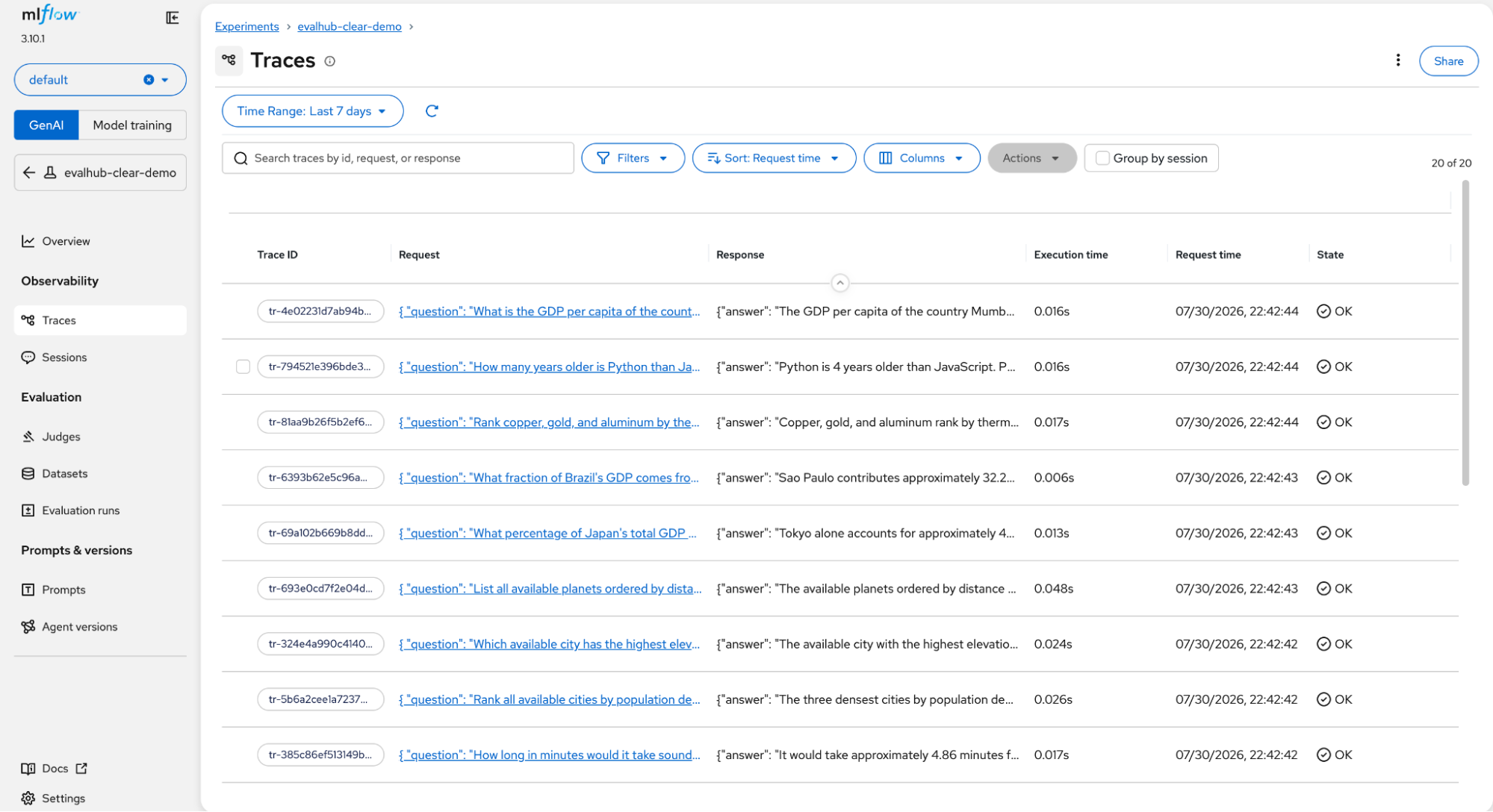
Traces found: 8

You can also verify visually in the MLflow UI, as shown in Figure 1: Select the default workspace, open the research agent traces experiment, and switch to the Traces tab (under GenAI).

Step 3: Deploy EvalHub on OpenShift AI

EvalHub orchestrates evaluation jobs as OpenShift jobs. It accepts job submissions via a REST API, creates pods running the CLEAR adapter container image, and collects results. The adapter pod connects to MLflow (running on the same cluster) to fetch traces and save evaluation artifacts.

Follow the official guides to deploy EvalHub:

• EvalHub Installation Guide
• EvalHub on OpenShift AI
• EvalHub custom resource reference

EvalHub is managed by the TrustyAI Operator, which is included with Red Hat OpenShift AI. If the TrustyAI Operator isn't yet installed on your cluster, follow the TrustyAI installation guide.

Once you deploy EvalHub, register the ibm-clear provider. This tells EvalHub which adapter image to use when scheduling CLEAR evaluation jobs. The provider definition is maintained in eval hub contrib.

Verify EvalHub is running

EVALHUB_ROUTE=$(oc get route evalhub -n redhat-ods-applications -o jsonpath='{.spec.host}')
EVALHUB_URL="https://${EVALHUB_ROUTE}"

# Health check
curl -sk "${EVALHUB_URL}/api/v1/health"

Confirm the ibm-clear provider is registered:

curl -sk "${EVALHUB_URL}/api/v1/providers" \
  -H "Authorization: Bearer $(oc whoami -t)" \
  -H "X-Tenant: redhat-ods-applications"

You should see ibm-clear in the list of available providers.

Create the judge LLM API key secret

The CLEAR adapter needs credentials for the judge LLM. Store them as an OpenShift secret that EvalHub will mount into the adapter pod:

oc create secret generic judge-llm-api-key \
  -n redhat-ods-applications \
  --from-literal=api-key=<YOUR_API_KEY> \
  --from-literal=OPENAI_API_KEY=<YOUR_API_KEY>

The secret needs both keys because api-key is what EvalHub's credential resolver reads (mounted at /var/run/secrets/model/api-key), and OPENAI_API_KEY is what LiteLLM uses when routing calls through the OpenAI-compatible interface.

Note: If you use a provider that requires a different environment variable (such as GOOGLE_API_KEY for Gemini or ANTHROPIC_API_KEY for Claude), add that key to the secret as well.

Step 4: Understanding CLEAR evaluation modes

Before configuring the job, it's important to understand what CLEAR evaluates and how.

Analysis types

CLEAR provides 2 complementary analysis types:

• Step-by-step: Evaluates individual LLM interactions using CLEAR methodology. Use case: Understanding agent-level quality issues per node.
• Full trajectory: Evaluates complete task trajectories for success, quality, and rubric-based scoring. Use case: Assessing overall task completion and quality.

The EvalHub adapter currently runs step-by-step analysis, evaluating each LLM interaction independently and discovering recurring issues across all traces.

Standard mode for LLM error analysis

In standard mode (separate_tools: false), CLEAR evaluates each agent step holistically. If an LLM call produces both reasoning text and tool calls, they're scored together as a single interaction. The judge assesses the overall quality of the response: Was the reasoning sound? Was the tool choice appropriate? Did the output address the input?

This mode works well for general-purpose evaluation where you want a single quality assessment per step.

SPARC mode for tool-level LLM error analysis)

Semantic Pre-execution Analysis for Reliable Calls (SPARC) is a dedicated tool call evaluation engine integrated into CLEAR. Enable SPARC by setting separate_tools: true. In this mode, CLEAR's preprocessor splits tool call interactions into separate rows, then routes reasoning and tool calls to different evaluators:

• Reasoning rows: Text responses scored by the standard CLEAR judge.
• Tool call rows: Each function call is scored individually by the SPARC engine for aspects such as argument correctness and tool selection appropriateness.

Both standard and SPARC modes evaluate tool calls, but SPARC does it more rigorously. Rather than folding a step's tool calls into one holistic score, it evaluates each tool call separately with a dedicated reflection engine.

This gives clearer feedback: you can see whether your agent reasons well but picks the wrong tool, or calls the right tool with malformed arguments.

Use SPARC when:

• Your agent makes structured function calls (API requests, database queries, tool invocations).
• You want to separately track tool usage quality versus reasoning quality over time.
• You're debugging tool selection issues hidden in combined evaluation.

Note that SPARC is slower than standard mode. Because it evaluates each tool call as its own row with a dedicated reflection engine, it issues roughly twice as many LLM calls as a standard run over the same traces.

We'll submit both evaluations in this tutorial so you can compare the results.

Step 5: Configure and submit the evaluation job

Use the following payload structure to submit the evaluation job to EvalHub:

{
  "name": "clear-research-agent-eval",
  "model": {
    "url": "<YOUR_MODEL_ENDPOINT>",
    "name": "<YOUR_MODEL_NAME>",
    "auth": {
      "secret_ref": "judge-llm-api-key"
    }
  },
  "experiment_name": "clear-eval-results",
  "benchmarks": [
    {
      "id": "agentic-evaluation",
      "provider_id": "ibm-clear",
      "parameters": {
        "mlflow_traces_experiment_name": "research-agent-traces",
        "mlflow_experiment_name": "clear-eval-results",
        "mlflow_workspace": "default",
        "eval_model_name": "<YOUR_MODEL_NAME>",
        "provider": "openai",
        "inference_backend": "litellm",
        "separate_tools": false,
        "agent_framework": "langgraph",
        "observability_framework": "mlflow"
      }
    }
  ]
}

For example, use the following configuration for Gemini 2.5 Flash:

{
  "model": {
    "url": "https://generativelanguage.googleapis.com/v1beta/openai",
    "name": "gemini-2.5-flash",
    "auth": {"secret_ref": "judge-llm-api-key"}
  }
}

Alternatively, use the following configuration for a self-hosted vLLM endpoint:

{
  "model": {
    "url": "http://vllm-server.my-namespace.svc:8000/v1",
    "name": "meta-llama/Llama-3.1-8B-Instruct",
    "auth": {"secret_ref": "judge-llm-api-key"}
  }
}

Parameter reference

• model.url: OpenAI-compatible /v1 base URL for the judge LLM
• model.name: Model identifier passed in API calls
• model.auth.secret_ref: Name of the OpenShift secret containing the API key
• experiment_name: Top-level MLflow experiment for saving results
• mlflow_traces_experiment_name: MLflow experiment to fetch input traces from
• mlflow_experiment_name: MLflow experiment to save evaluation results to
• mlflow_workspace: MLflow workspace (maps to OpenShift namespace for RBAC)
• eval_model_name: Bare model name (CLEAR constructs {provider}/{eval_model_name} for LiteLLM)
• provider: LiteLLM provider prefix (for example, openai, anthropic, gemini)
• inference_backend: litellm (default), langchain, or endpoint (legacy)
• separate_tools: false equals standard mode, true equals SPARC (tool call analysis)
• agent_framework: langgraph or crewai tells CLEAR how to parse trace spans
• observability_framework: mlflow or langfuse sets trace source format

Supported framework combinations

• langgraph with mlflow: Supported
• langgraph with langfuse: Supported
• crewai with langfuse: Supported
• crewai with mlflow: Not supported

When using MLflow as the observability framework, only langgraph is supported.

About inference_backend

• litellm (default, recommended): The adapter sets model.url as OPENAI_BASE_URL. LiteLLM routes all judge calls through it. Supports any OpenAI-compatible endpoint.
• langchain: Uses LangChain as the inference backend for judge calls.
• endpoint (legacy): Passes model.url directly as endpoint_url to CLEAR's internal inference. Use litellm for new deployments.

How EvalHub connects to MLflow

When EvalHub creates the adapter pod, a sidecar automatically injects:

• MLFLOW_TRACKING_URI: Pointing to the in-cluster MLflow service
• MLFLOW_TRACKING_TOKEN: From the pod's service account
• MLFLOW_WORKSPACE: Set to the tenant namespace

The mlflow_workspace parameter in the job JSON tells the adapter which workspace to use for fetching traces and saving results (overriding the sidecar's default). This is necessary when your traces live in a workspace different from the namespace where the job pod runs.

Submit the standard evaluation

Run the following command to submit the standard evaluation job to EvalHub:

TOKEN=$(oc whoami -t)
curl -sk -X POST "${EVALHUB_URL}/api/v1/evaluations/jobs" \
  -H "Authorization: Bearer ${TOKEN}" \
  -H "X-Tenant: redhat-ods-applications" \
  -H "Content-Type: application/json" \
  -d '{
    "name": "clear-standard-eval",
    "model": {
      "url": "<YOUR_MODEL_ENDPOINT>",
      "name": "<YOUR_MODEL_NAME>",
      "auth": {"secret_ref": "judge-llm-api-key"}
    },
    "experiment_name": "clear-eval-results",
    "benchmarks": [{
      "id": "agentic-evaluation",
      "provider_id": "ibm-clear",
      "parameters": {
        "mlflow_traces_experiment_name": "research-agent-traces",
        "mlflow_experiment_name": "clear-eval-results",
        "mlflow_workspace": "default",
        "eval_model_name": "<YOUR_MODEL_NAME>",
        "provider": "openai",
        "inference_backend": "litellm",
        "separate_tools": false,
        "agent_framework": "langgraph",
        "observability_framework": "mlflow"
      }
    }]
  }'

The response contains the job ID:

{"id": "eval-a1b2c3d4", "state": "pending"}

Submit the SPARC evaluation

Submit a second job with separate_tools: true to compare the results:

 curl -sk -X POST "${EVALHUB_URL}/api/v1/evaluations/jobs" \
  -H "Authorization: Bearer ${TOKEN}" \
  -H "X-Tenant: redhat-ods-applications" \
  -H "Content-Type: application/json" \
  -d '{
    "name": "clear-sparc-eval",
    "model": {
      "url": "<YOUR_MODEL_ENDPOINT>",
      "name": "<YOUR_MODEL_NAME>",
      "auth": {"secret_ref": "judge-llm-api-key"}
    },
    "experiment_name": "clear-eval-sparc-results",
    "benchmarks": [{
      "id": "agentic-evaluation",
      "provider_id": "ibm-clear",
      "parameters": {
        "mlflow_traces_experiment_name": "research-agent-traces",
        "mlflow_experiment_name": "clear-eval-sparc-results",
        "mlflow_workspace": "default",
        "eval_model_name": "<YOUR_MODEL_NAME>",
        "provider": "openai",
        "inference_backend": "litellm",
        "separate_tools": true,
        "agent_framework": "langgraph",
        "observability_framework": "mlflow"
      }
    }]
  }'

Monitor job status

Evaluation runs as a background OpenShift job; the adapter pod processes all traces, calls the judge model for each interaction, and reports back when complete. Check status with:

JOB_ID="eval-a1b2c3d4"
curl -sk "${EVALHUB_URL}/api/v1/evaluations/jobs/${JOB_ID}" \
  -H "Authorization: Bearer ${TOKEN}" \
  -H "X-Tenant: redhat-ods-applications" \
  | python3 -c "import json,sys; j=json.load(sys.stdin); print(f'State: {j[\"status\"][\"state\"]}')"

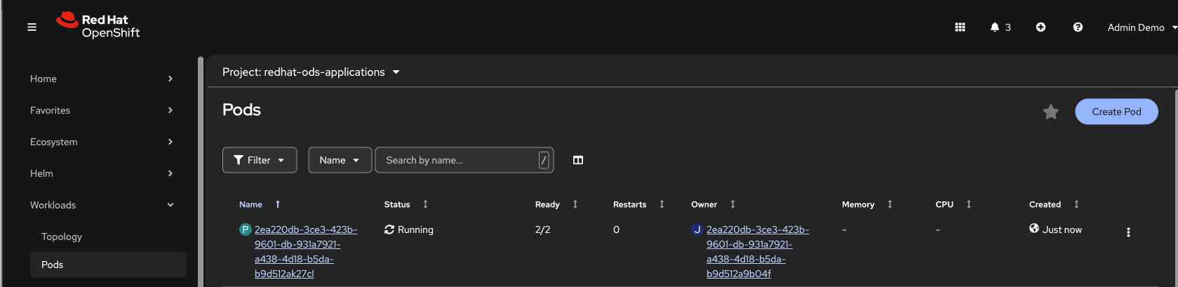
You can monitor the adapter pod status in the Red Hat OpenShift console, as shown in Figure 2.

Review active step-analysis logs from the adapter pod in the Red Hat OpenShift console, as shown in Figure 3.

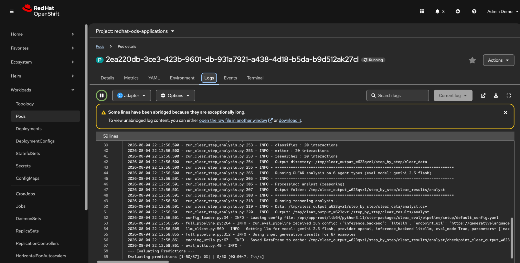
The adapter pod starts running, fetches traces from MLflow, and begins evaluating each agent's interactions against the judge model. For 8 traces with roughly 30 spans each, expect 5 to 10 minutes per job depending on the judge model's latency.

Step 6: View results in MLflow

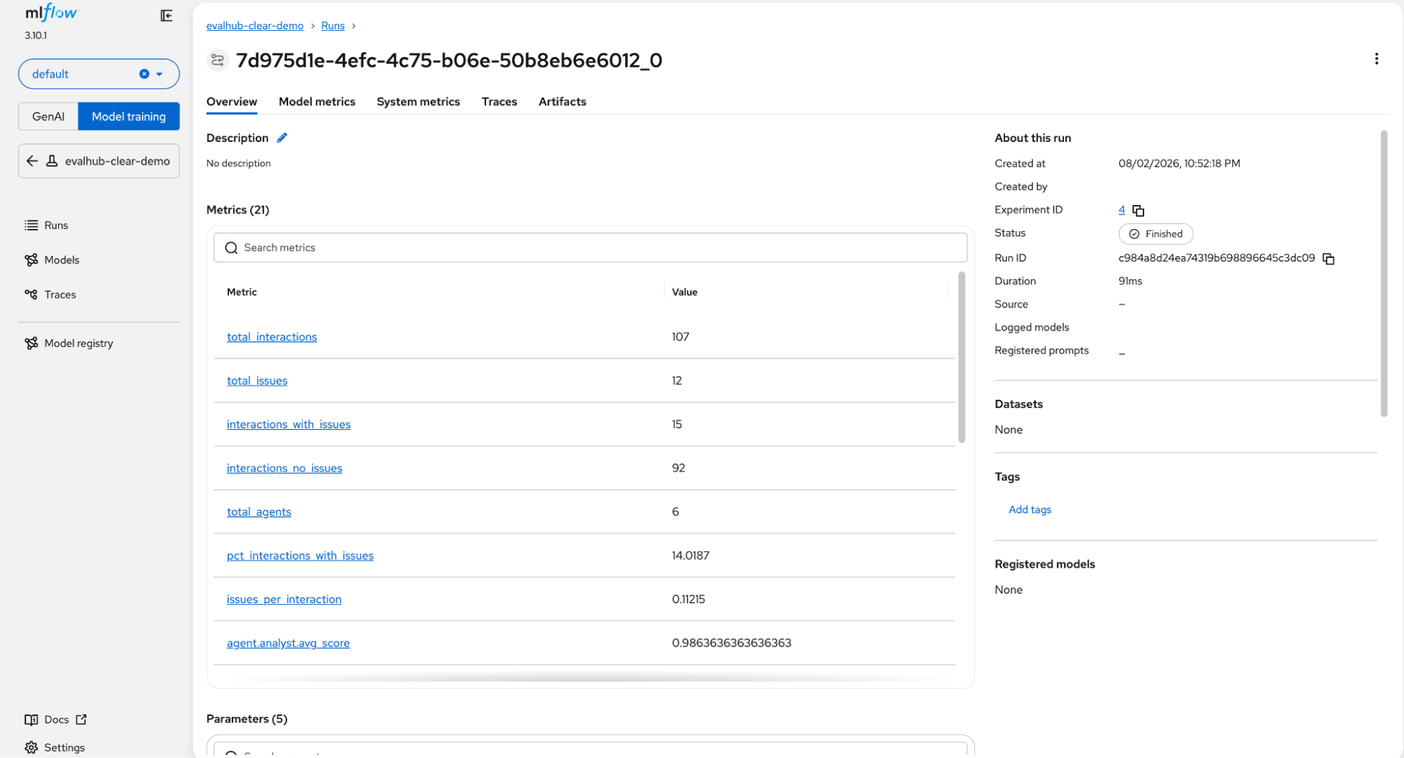
Once both jobs complete, open the MLflow UI, navigate to the default workspace, and open the evalhub-clear-demo experiment, as shown in Figure 4.

Metrics (example values)

The evaluation run logs the following key metrics in MLflow:

• overall_score: Average across all agent types (0.0 to 1.0). Higher is better.
• agent.research_node.avg_score: Score for the research step to identify weak points.
• agent.analysis_node.avg_score: Score for the analysis or synthesis step.
• total_issues: Unique failure patterns discovered across all traces.
• total_interactions: Total LLM interactions analyzed.

When you compare standard versus SPARC runs on the same traces, differences in scores reveal whether issues stem from tool usage or reasoning. If SPARC scores are higher, it suggests tool calls are correct, but the agent's underlying reasoning needs refinement.

Artifacts

The evaluation run generates and saves the following artifacts in MLflow:

• clear_results.json: Full structured results with per-interaction scores and the complete issue catalog. Use this for programmatic analysis or CI/CD gates.
• metrics_summary.json: Aggregated metrics in a compact JSON format.
• clear_results.html: Interactive HTML dashboard with visualizations and drill-downs.
• clear_results.dashboard_data.json: Data backing the HTML dashboard.

Viewing the HTML dashboard

Download the HTML artifact from MLflow and open it in your browser:

# Get the run ID from the EvalHub job response (or find it in MLflow UI)
RUN_ID="<your run id>"
# Download the HTML report
curl -sk "${MLFLOW_TRACKING_URI}/api/2.0/mlflow/artifacts/artifacts/${RUN_ID}/artifacts/clear_results.html" \
  -H "Authorization: Bearer ${MLFLOW_TOKEN}" \
  -H "X-MLFLOW-WORKSPACE: default" \
  -o clear_results.html
# Open in browser
open clear_results.html   # macOS
# xdg-open clear_results.html  # Linux

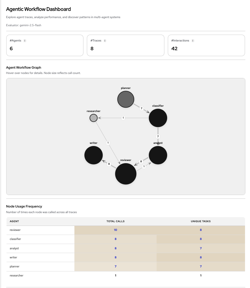
Alternatively, in the MLflow UI: Navigate to the run, click the Artifacts tab, select clear_results.html, and click Download. The top section of the HTML report displays workflow metrics and node frequencies, as shown in Figure 5.

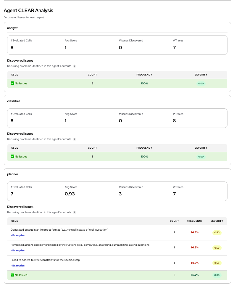
Detailed per-agent analysis metrics and issue breakdowns for the analyst, classifier, and planner agents appear in Figure 6.

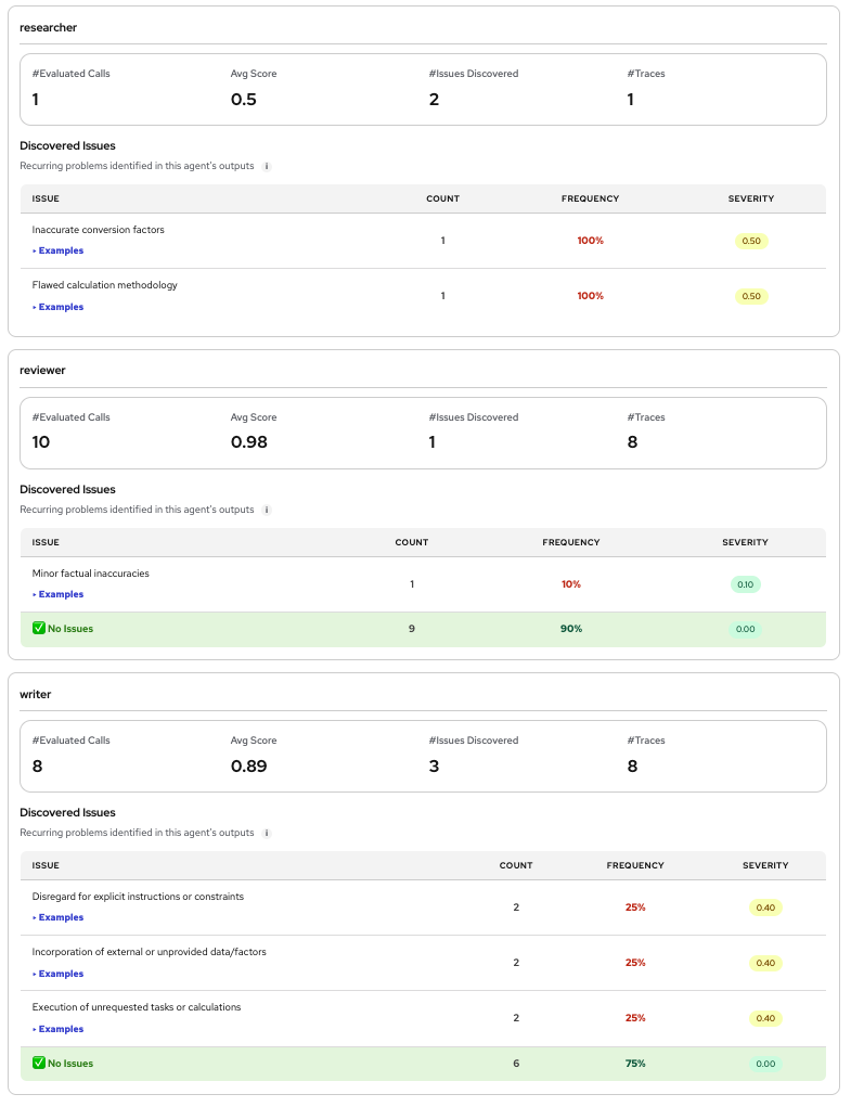
Review the breakdown of performance metrics and recurring issue logs for the researcher, reviewer, and writer agents in Figure 7.

The HTML dashboard shows:

• Per-agent score distributions: Which agent types are weakest
• Issues catalog: Recurring failure patterns ranked by frequency
• Individual interaction evaluations: The judge's reasoning for each score
• Score distributions: How scores vary across interactions

Reading the results

CLEAR scores each agent type independently (based on span names in your traces), then averages them into an overall score. The lowest-scoring agent type tells you where to focus improvement efforts: examine the issues CLEAR found for that type, check whether retrieval surfaces relevant context, and test prompt adjustments.

When you compare standard with SPARC mode, the 2 modes track interactions differently. In standard mode, each LLM call is a single interaction; if that call produces both reasoning and multiple tool calls, they're scored together as 1 unit. In SPARC mode, each tool call is split into its own interaction row, so the total interaction count and per-agent evaluation counts will differ between runs.

When you compare scores: if SPARC produces higher reasoning scores, it suggests tool calls were pulling down the combined score in standard mode. If SPARC reveals low scores specifically on tool-call rows, your agent might be selecting wrong tools or passing malformed arguments—issues hidden in standard mode's combined scoring.

Tips and best practices

Keep these practical tips in mind as you tune your evaluation pipeline:

• Start with standard mode, then try SPARC. Standard mode gives you a single quality score per step. If you notice tool-related issues in the results, enable SPARC to get a granular tool versus reasoning breakdown.
• Pin your judge model. Small model updates shift scores. Use a specific version (for example, gemini-2.5-flash instead of gemini-latest) so score changes reflect your agent's behavior, not the judge's.
• Track scores across runs. Each CLEAR evaluation creates a new MLflow run. Use MLflow's comparison view to track agent.<name>.avg_score over time as you iterate on prompts, retrieval, or tool definitions.
• Limit trace volume during iteration. Set "max_examples_to_analyze": 5 in parameters to keep evaluation runs under a minute while tuning.
• Use the same workspace consistently. Your traces and results should live in the same MLflow workspace. If you use a workspace other than default, verify that the EvalHub service account has the MLflow integration ClusterRole bound in the corresponding namespace.

Wrap up

In this tutorial, you:

1. Deployed MLflow on Red Hat OpenShift AI as the trace and result store.
2. Uploaded agent traces: Structured records of LLM calls, tool invocations, and reasoning steps from a multistep research agent.
3. Deployed EvalHub as the evaluation orchestrator, configured with the IBM CLEAR adapter.
4. Submitted evaluation jobs in both standard and SPARC modes through the EvalHub REST API.
5. Viewed results in MLflow: Per-agent scores, a ranked issue catalog, and an interactive HTML dashboard, all stored as MLflow artifacts for comparison and tracking over time.

The entire flow runs on-cluster with no external dependencies beyond the judge LLM endpoint. You can integrate evaluation into CI/CD pipelines using the evalhub CLI, gate deployments on score thresholds, and track quality regressions across agent iterations.

Take control of your agentic AI pipeline

Bridge the evaluation gap and build reliable AI agents with confidence. Test-drive the platform today in the Developer Sandbox or start a 60-day OpenShift AI trial to see how Red Hat provides the open, scalable foundation you need to train, deploy, and continuously evaluate AI models across the hybrid cloud. Explore the full Red Hat portfolio to power your end-to-end MLOps strategy.

Resources

Red Hat OpenShift AI:

• Install and configure MLflow, Red Hat OpenShift AI 3.4

EvalHub:

• EvalHub documentation

IBM CLEAR:

• IBM CLEAR: Comprehensive LLM Evaluation and Analysis for Reasoning
• CLEAR MLflow tracing requirements

MLflow:

• MLflow documentation
• MLflow tracing guide

Appendix A: Generating and uploading agent traces to MLflow

This appendix covers 2 approaches:

• Uploading pre-recorded trace files using the EvalHub SDK's MLflow client.
• Generating traces programmatically using the MLflow SDK (simulating an agent).

Environment setup

export MLFLOW_TRACKING_URI="https://<your-mlflow-route>/mlflow"
export MLFLOW_TRACKING_TOKEN="$(oc whoami -t)"
export MLFLOW_WORKSPACE="default"

# Only needed if your cluster uses self-signed TLS certificates (e.g., test environments)
export MLFLOW_TRACKING_INSECURE_TLS="true"

Option 1: Upload prerecorded trace files

If you have trace JSON files exported from a previous MLflow experiment or generated by a LangGraph agent, upload them directly using the EvalHub SDK:

import os
import sys
import time
from pathlib import Path

from evalhub.adapter.mlflow import MlflowClient

client = MlflowClient()

EXPERIMENT_NAME = "research agent traces"
exp_id = client.get_or_create_experiment(EXPERIMENT_NAME)
print(f"Experiment: {EXPERIMENT_NAME} (id={exp_id})")

traces_dir = Path("raw_traces")
trace_files = sorted(traces_dir.glob("*.json"))[:8]
print(f"Uploading {len(trace_files)} trace files...")

for i, f in enumerate(trace_files, 1):
    request_id = client.traces.upload_trace_file(exp_id, f)
    print(f"  [{i}/{len(trace_files)}] {request_id} ({f.name})")
    time.sleep(0.5)

print(f"\nDone. {len(trace_files)} traces uploaded to '{EXPERIMENT_NAME}'.")

Option 2: Generate traces programmatically

This script simulates a multistep research agent and records traces using the MLflow SDK. Each trace has the structure CLEAR expects: an AGENT root span with CHAIN, CHAT_MODEL, and TOOL children.

import os
import json
import mlflow
from mlflow.entities import SpanType
from mlflow.tracking.request_header.abstract_request_header_provider import (
    RequestHeaderProvider,
)
from mlflow.tracking.request_header.registry import _request_header_provider_registry


class WorkspaceHeaderProvider(RequestHeaderProvider):
    """Injects X-MLFLOW-WORKSPACE header for OpenShift AI MLflow."""

    def in_context(self):
        return True

    def request_headers(self):
        return {"X-MLFLOW-WORKSPACE": os.environ.get("MLFLOW_WORKSPACE", "default")}


_request_header_provider_registry.register(WorkspaceHeaderProvider)

mlflow.set_tracking_uri(os.environ["MLFLOW_TRACKING_URI"])
experiment = mlflow.set_experiment("research agent traces")

SCENARIOS = [
    {
        "question": "Which available city has the highest elevation? Convert to feet.",
        "tool_calls": [
            {"name": "knowledge_lookup", "args": {"topic": "tokyo"}},
            {"name": "knowledge_lookup", "args": {"topic": "sao paulo"}},
            {"name": "unit_converter", "args": {"value": 760, "from_unit": "meters", "to_unit": "feet"}},
        ],
        "tool_results": [
            '{"type": "city", "elevation_m": 40, "country": "Japan"}',
            '{"type": "city", "elevation_m": 760, "country": "Brazil"}',
            "760.0 meters = 2493.44 feet",
        ],
        "answer": "São Paulo has the highest elevation at 760m (2493.44 feet).",
    },
    {
        "question": "What is the GDP per capita of the largest city by population?",
        "tool_calls": [
            {"name": "knowledge_lookup", "args": {"topic": "mumbai"}},
            {"name": "knowledge_lookup", "args": {"topic": "tokyo"}},
            {"name": "calculator", "args": {"expression": "1920000000000 / 13960000"}},
        ],
        "tool_results": [
            '{"type": "city", "population": 20667000, "gdp_billion_usd": 368}',
            '{"type": "city", "population": 13960000, "gdp_billion_usd": 1920}',
            "137535.82",
        ],
        "answer": "Mumbai is the largest city (20.7M people) with GDP per capita of ~$17,800.",
    },
    {
        "question": "Compare the timezone differences between Sydney and New York.",
        "tool_calls": [
            {"name": "knowledge_lookup", "args": {"topic": "sydney"}},
            {"name": "knowledge_lookup", "args": {"topic": "new york"}},
            {"name": "calculator", "args": {"expression": "11 minus (negative 5)"}},
        ],
        "tool_results": [
            '{"type": "city", "timezone": "UTC+11"}',
            '{"type": "city", "timezone": "UTC minus 5"}',
            "16",
        ],
        "answer": "Sydney is 16 hours ahead of New York (UTC+11 vs UTC minus 5).",
    },
    {
        "question": "Which city has the best GDP to area ratio?",
        "tool_calls": [
            {"name": "knowledge_lookup", "args": {"topic": "tokyo"}},
            {"name": "knowledge_lookup", "args": {"topic": "paris"}},
            {"name": "knowledge_lookup", "args": {"topic": "london"}},
            {"name": "calculator", "args": {"expression": "max(1920/2194, 850/105, 1100/1572)"}},
        ],
        "tool_results": [
            '{"type": "city", "area_km2": 2194, "gdp_billion_usd": 1920}',
            '{"type": "city", "area_km2": 105, "gdp_billion_usd": 850}',
            '{"type": "city", "area_km2": 1572, "gdp_billion_usd": 1100}',
            "8.095",
        ],
        "answer": "Paris has the best GDP to area ratio at $8.1B/km² due to its compact area.",
    },
    {
        "question": "What is the average temperature across all available cities?",
        "tool_calls": [
            {"name": "knowledge_lookup", "args": {"topic": "tokyo"}},
            {"name": "knowledge_lookup", "args": {"topic": "new york"}},
            {"name": "knowledge_lookup", "args": {"topic": "paris"}},
            {"name": "knowledge_lookup", "args": {"topic": "mumbai"}},
            {"name": "calculator", "args": {"expression": "(16.3+12.9+12.4+27.2)/4"}},
        ],
        "tool_results": [
            '{"type": "city", "avg_temp_celsius": 16.3}',
            '{"type": "city", "avg_temp_celsius": 12.9}',
            '{"type": "city", "avg_temp_celsius": 12.4}',
            '{"type": "city", "avg_temp_celsius": 27.2}',
            "17.2",
        ],
        "answer": "The average temperature across 4 cities is 17.2°C.",
    },
    {
        "question": "Rank the top 3 cities by population density.",
        "tool_calls": [
            {"name": "knowledge_lookup", "args": {"topic": "mumbai"}},
            {"name": "knowledge_lookup", "args": {"topic": "paris"}},
            {"name": "knowledge_lookup", "args": {"topic": "tokyo"}},
            {"name": "calculator", "args": {"expression": "20667000/603, 2161000/105, 13960000/2194"}},
        ],
        "tool_results": [
            '{"type": "city", "population": 20667000, "area_km2": 603}',
            '{"type": "city", "population": 2161000, "area_km2": 105}',
            '{"type": "city", "population": 13960000, "area_km2": 2194}',
            "34274, 20581, 6362",
        ],
        "answer": "1. Mumbai (34,274/km²), 2. Paris (20,581/km²), 3. Tokyo (6,362/km²).",
    },
    {
        "question": "Which city would be most affected by a 2m sea level rise?",
        "tool_calls": [
            {"name": "knowledge_lookup", "args": {"topic": "new york"}},
            {"name": "knowledge_lookup", "args": {"topic": "mumbai"}},
            {"name": "knowledge_lookup", "args": {"topic": "london"}},
        ],
        "tool_results": [
            '{"type": "city", "elevation_m": 10}',
            '{"type": "city", "elevation_m": 14}',
            '{"type": "city", "elevation_m": 11}',
        ],
        "answer": "New York (10m elevation) would be most affected, followed by London (11m).",
    },
    {
        "question": "Calculate the total GDP of all cities in the UTC+ timezones.",
        "tool_calls": [
            {"name": "knowledge_lookup", "args": {"topic": "tokyo"}},
            {"name": "knowledge_lookup", "args": {"topic": "paris"}},
            {"name": "knowledge_lookup", "args": {"topic": "sydney"}},
            {"name": "knowledge_lookup", "args": {"topic": "mumbai"}},
            {"name": "calculator", "args": {"expression": "1920+850+440+368"}},
        ],
        "tool_results": [
            '{"type": "city", "timezone": "UTC+9", "gdp_billion_usd": 1920}',
            '{"type": "city", "timezone": "UTC+1", "gdp_billion_usd": 850}',
            '{"type": "city", "timezone": "UTC+11", "gdp_billion_usd": 440}',
            '{"type": "city", "timezone": "UTC+5:30", "gdp_billion_usd": 368}',
            "3578",
        ],
        "answer": "Total GDP of UTC+ cities: $3,578 billion (Tokyo, Paris, Sydney, Mumbai).",
    },
]

for i, scenario in enumerate(SCENARIOS):
    trace_name = f"research_agent_q{i+1:03d}"

    with mlflow.start_span(name=trace_name, span_type=SpanType.AGENT) as root:
        root.set_inputs({"question": scenario["question"]})

        # LangGraph orchestration node
        with mlflow.start_span(name="LangGraph", span_type=SpanType.CHAIN) as chain:
            chain.set_inputs({"question": scenario["question"], "messages": []})

            # Research node: LLM decides which tools to call
            with mlflow.start_span(name="research_node", span_type="CHAT_MODEL") as llm1:
                llm1.set_inputs({
                    "messages": [
                        {"role": "system", "content": "You are a research agent with access to tools."},
                        {"role": "user", "content": scenario["question"]},
                    ]
                })
                llm1.set_attribute("gen_ai.operation.name", "chat")
                llm1.set_attribute("gen_ai.request.model", "gpt 4.1 mini")
                llm1.set_attribute("gen_ai.system", "openai")
                llm1.set_outputs({
                    "choices": [{
                        "message": {
                            "role": "assistant",
                            "content": "",
                            "tool_calls": [
                                {"name": tc["name"], "arguments": json.dumps(tc["args"]),
                                 "id": f"call_{i}_{j}", "type": "function"}
                                for j, tc in enumerate(scenario["tool_calls"])
                            ],
                        }
                    }]
                })

            # Tool execution spans
            for j, (tc, result) in enumerate(
                zip(scenario["tool_calls"], scenario["tool_results"])
            ):
                with mlflow.start_span(name=tc["name"], span_type=SpanType.TOOL) as tool:
                    tool.set_inputs(tc["args"])
                    tool.set_outputs({"result": result})

            # Analysis node: LLM synthesizes final answer
            with mlflow.start_span(name="analysis_node", span_type="CHAT_MODEL") as llm2:
                llm2.set_inputs({
                    "messages": [
                        {"role": "system", "content": "Synthesize a final answer from research."},
                        {"role": "user", "content": scenario["question"]},
                        {"role": "assistant", "content": f"Research complete. Findings: {scenario['tool_results']}"},
                    ]
                })
                llm2.set_attribute("gen_ai.operation.name", "chat")
                llm2.set_attribute("gen_ai.request.model", "gpt 4.1 mini")
                llm2.set_attribute("gen_ai.system", "openai")
                llm2.set_outputs({
                    "choices": [{
                        "message": {"role": "assistant", "content": scenario["answer"]}
                    }]
                })

            chain.set_outputs({"answer": scenario["answer"]})

        root.set_outputs({"answer": scenario["answer"]})

    print(f"[{i+1}/{len(SCENARIOS)}] Created trace: {trace_name}")

print(f"\nDone. {len(SCENARIOS)} traces created in '{experiment.name}'.")

What the traces look like

Each trace has this span hierarchy:

AGENT (research agent q001)
  CHAIN (LangGraph)
    CHAT_MODEL (research node)     LLM decides tool calls
    TOOL (knowledge lookup)         Tool execution
    TOOL (unit converter)           Tool execution
    CHAT_MODEL (analysis node)     LLM synthesizes answer

CLEAR's preprocessor identifies LLM call spans using these rules (from process_mlflow_traces.py):

• A span is scored as an LLM call if any of these are true:
  • span_type is CHAT_MODEL, MODEL, or GENERATION
  • Has a gen_ai.operation.name attribute
  • Has choices in its outputs dict

Span types summary

• CHAT_MODEL: Chat completion call (scored by CLEAR)
• MODEL: Generic model call (scored by CLEAR)
• GENERATION: Text generation call (scored by CLEAR)
• AGENT: Root-level orchestration (not scored, wrapper)
• CHAIN: Sequential processing node (not scored, wrapper)
• TOOL: Tool execution (scored by CLEAR in SPARC mode only)

For full tracing requirements, see the CLEAR MLflow Tracing Requirements documentation.

Alternative: Auto-generated traces with LangGraph

If your agent is already running with LangGraph and MLflow tracing:

import mlflow

mlflow.langchain.autolog()
mlflow.set_tracking_uri(os.environ["MLFLOW_TRACKING_URI"])
mlflow.set_experiment("research agent traces")

# Run your agent, traces are created automatically
result = agent.invoke({"question": "What is the capital of France?"})