Retrieval-augmented generation (RAG) is a well-worn path by now. Parse the data, chunk it, embed the chunks, retrieve the ones closest to the question, stuff them into the prompt, and let the model answer. You've built this. The shape is familiar. Or if you haven't, this Red Hat primer on RAG and tuning is a good place to start.
The part that not a lot of people tell you up front is that the path has a dozen different knobs. Chunk size, overlap, how many chunks you retrieve, whether you retrieve by keyword, vector, or both—the combination that works best is different for every dataset. The usual workflow is to pick a chunk size from a tutorial, set top-k high to be safe, eyeball a few answers, and ship it. That ships a guess.
On a small, locally hosted model like the ones you usually run on your laptop, a bad guess hurts significantly more. A smaller model has less capacity to sort the right detail out of a pile of lookalikes. If you feed it a massive block of loosely related context, it will confidently pull the wrong one, leaving you to spend hours nudging knobs to fix it by feel.
So I built a small demo that makes that failure visible, then fixes it by running a set of evals comparing a naive baseline against the config AutoRAG picks.
The mental model
A quick note on scope
This demo runs the actual AutoRAG optimization logic, but it is a focused implementation. It is not the full open source AutoRAG project or the Red Hat platform feature of the same name. We’ll cover those production differences later.
RAG is an open-book exam for the model. Instead of answering from memory, which is stale and prone to hallucination, it looks things up in your "book," your data, at answer time. Naive RAG, the default setup where you pick one configuration up front and never change it, hands the model one fixed way of finding pages. AutoRAG tunes how it finds pages: it tries many different combinations of settings, scores each one against a set of questions based on your own data where the correct answer is already known, and keeps the configuration that found the right pages most reliably.
The insight that makes hand-tuning miserable is that there is no universal best RAG pipeline. The best one is a function of your data and your queries, so it can't ship as a default. It has to be discovered per corpus. And the winner is the output of running the evaluation, not something you have before you run it. In the demo, the tuned configuration literally stays locked until you run the sweep, which is the honest version of how this works.
Inside the AutoRAG loop: Fast, deterministic retrieval scoring without LLMs
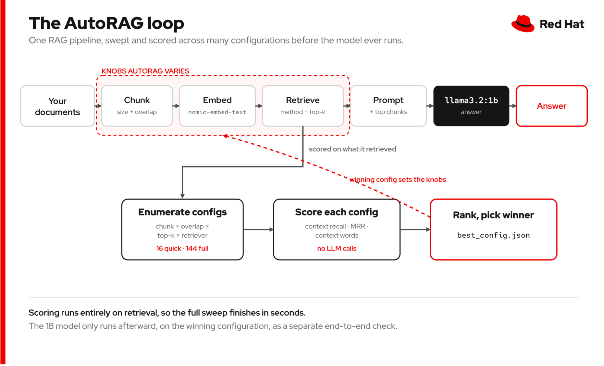
The demo tests four settings: how big each chunk of text is, how much neighboring chunks overlap, how many chunks get handed to the model, and how the search itself works. That last one comes in three flavors: semantic search, which matches on meaning, so a question about "refunds" can find a passage about "reimbursements"; keyword search, which matches on the exact words, the way a classic search engine does; or hybrid, which runs both and merges the results into one list. The demo tests a fixed menu of combinations rather than a random sample: 16 configurations in the quick sweep, 144 in the full one.
For each configuration, it builds the index, embeds the chunks with nomic-embed-text, and runs retrieval over a 21-question evaluation set. Then it scores, and this is the part that makes the whole thing fast: the score uses no LLM calls at all. The AutoRAG process calculates three numbers per configuration:
context_recall: Did we retrieve the chunk that actually contains the answer?- MRR (Mean Reciprocal Rank): A measure of how high up in the result list the first relevant chunk appears, where a higher score means the answer is ranked closer to the top.
avg_ctx_words: How much text did we shove into the model, which is both noise and cost?
The composite is context_recall + 0.05·mrr − 0.00002·avg_ctx_words. Recall dominates, MRR breaks ties between configurations that both find the answer, and the tiny penalty on context size rewards a config that gets the answer in less text. Because none of this calls the model, sweeping all 144 configs takes seconds. In the context of our demo, the best one gets written to best_config.json.
Only then does the model enter. The end-to-end check is a separate step: run the 1-billion-parameter model on the naive baseline and on the winning configuration and compare the answers. Keep that split clear in your head. The sweep is deterministic retrieval scoring; the answer-quality comparison is a separate LLM pass, as illustrated in the loop diagram (Figure 1).
The corpus, and why it's mean on purpose
The data shown in the demo is a knowledge base of fictional but realistic bank card disputes and chargebacks: 16 Markdown policy documents covering filing timeframes, reason codes, provisional credit, liability limits, escalation, ATM disputes, digital wallet disputes, billing errors, and it is deliberately stuffed with colliding numbers. It includes several different "$50" and "$0" figures, "60 days" and "90 days" sitting near each other, and reason codes like 10.4, 13.1, 13.3, 13.6, 12.5.
That collision is the whole point. It's exactly the situation where a small model grabs the wrong figure if the retrieval is noisy, meaning it returns extra text that looks relevant but doesn't answer the question. The evaluation set is 21 questions, each with a reference answer and a specific phrase from the source document that the scorer checks for in the retrieved text. That expected phrase is what lets the scoring be deterministic with no LLM judge: either the chunk containing it came back or it didn't.
What the measurement turns up
The naive baseline is the configuration you'd reach for on day one: chunk size 250, no overlap, top-k 8, dense retrieval. The reasoning behind it is "don't chunk too aggressively, retrieve a lot to be safe." It produces about 1,367 words of context, and it does retrieve the answer. It retrieves the answer ranked first among eight chunks.
The config AutoRAG selects on this data is chunk size 150, overlap 30, top-k 3, dense. It hits 100% context recall, an MRR of 0.976, and about 165 context words. With the same recall as the naive configuration, it retrieves the answer ranked first among two chunks, and about 88% less context going into the model.
| Metric | Naive baseline | AutoRAG optimized | Result |
|---|---|---|---|
| Context recall (%) | 100% | 100% | Tie, recall saturates on a clean corpus |
| Mean reciprocal rank (MRR) | 0.976 | 0.976 | Tie, answer already ranks at top |
| Average context word count | 1,367 | 165 | -88% |
The 3-D Secure question shows the difference most clearly. Both configs answer correctly, but the naive setup finds the fact inside 1,367 words of retrieved text spread over 8 chunks, with 16 competing figures in the mix. AutoRAG finds the same answer in 2 chunks, using only 165 words and 4 competing figures, a quarter of the noise.
There is one caveat, which is also the main point of the demonstration. With the winning configuration, the 1-billion-parameter model still only gets about 12 of the 21 questions right under a strict substring match, partly because it phrases correct answers in ways the strict check misses. AutoRAG does not make a 1-billion-parameter model accurate. It narrows the gap, and it does so by giving the model clean, tight, correctly-ranked context instead of a pile of near-misses. Small models need good retrieval, honest evaluation, and later some inference-time scaling to do well. This demo covers the retrieval and evaluation part of that, shown end to end. No tuning pass on its own makes a 1-billion-parameter model reliable.
Calibrating expectations
This demo runs the core idea of AutoRAG: it tests four settings, checks every combination one by one, scores retrieval by looking for a specific expected phrase, and holds its vectors in memory.
The full implementations go further. The open source technique also tests embedding models, rerankers, query expansion methods such as HyDE, and prompt templates, and both it and the Red Hat OpenShift AI feature score answers with an LLM judge instead of a phrase check. For real workloads, the AutoRAG feature in Red Hat OpenShift AI is the version built for that job, with the wider search space, the real evaluation stack, and the governance around it.
Tune locally, scale the same code
The AutoRAG loop lets you experiment anywhere. You can start by running a sweep against a 1-billion-parameter model on your laptop using Ollama. When you’re ready to scale up to larger models, you simply switch your back end—the OpenAI-compatible code remains exactly the same, with no rewrite required.
Locally, the demo launches a browser-based web application where you can tweak sliders for individual configurations, run full sweeps, and track results on a leaderboard. You can even import your own TXT or MD files to test your data directly, comparing naive versus tuned results in real time. For a quick look at the impact on your data, try the import tab.
Moving from a laptop prototype to production is a matter of swapping the execution environment; your code remains consistent throughout:
- Model serving: Transition from local Ollama to model serving via vLLM on OpenShift AI.
- Infrastructure: Scale from a single process to distributed inference using llm-d.
- Data storage: Replace the in-memory vector store with a production-grade managed vector database.
- Evaluation: Graduate from simple phrase-checking to rigorous evaluations using the platform's EvalHub.
Because your application relies on OpenAI-compatible endpoints, your core code requires zero changes during these back-end swaps.
The production-grade version of this pipeline is Red Hat OpenShift AI. As a technology preview in OpenShift AI 3.4, it extends the AutoRAG concept by exploring a broader search space, including query expansion and reranking, and using a detailed evaluation stack. You can start by proving your methodology on a local 1-billion-parameter model, then seamlessly scale into the enterprise platform whenever you need production-level governance and capacity.
The takeaway
Optimizing RAG comes down to how cleanly you select context for your dataset, and manual knob-tuning quickly hits a wall.
Instead of relying on guesswork, automate your optimization: run a sweep, consult the leaderboard, and let the data choose your configuration. Using a smaller 1-billion-parameter model as your baseline is an excellent litmus test. Establishing effective retrieval and evaluation at this scale provides a practical foundation that can help simplify the process of moving to larger, more complex models.
Resources: