Populate a data science project

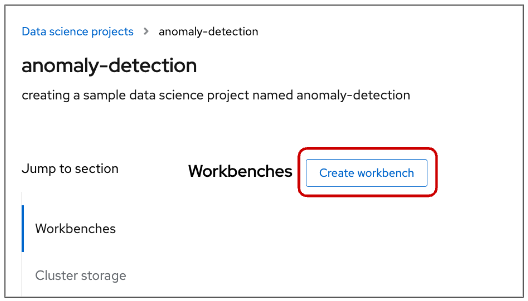
 Add a workbench by clicking the Create workbench button (Figure 6.)

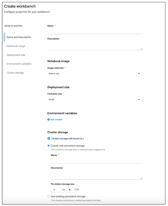
On the Create workbench page, complete the following information. Note: Not all fields are required. (Figure 7)

• Name
• Description
• Notebook image
• Deployment size (container size)
• Environment variables
• Cluster storage name
• Cluster storage description
• Persistent storage size

Once you have entered the information for your workbench, click Create. 

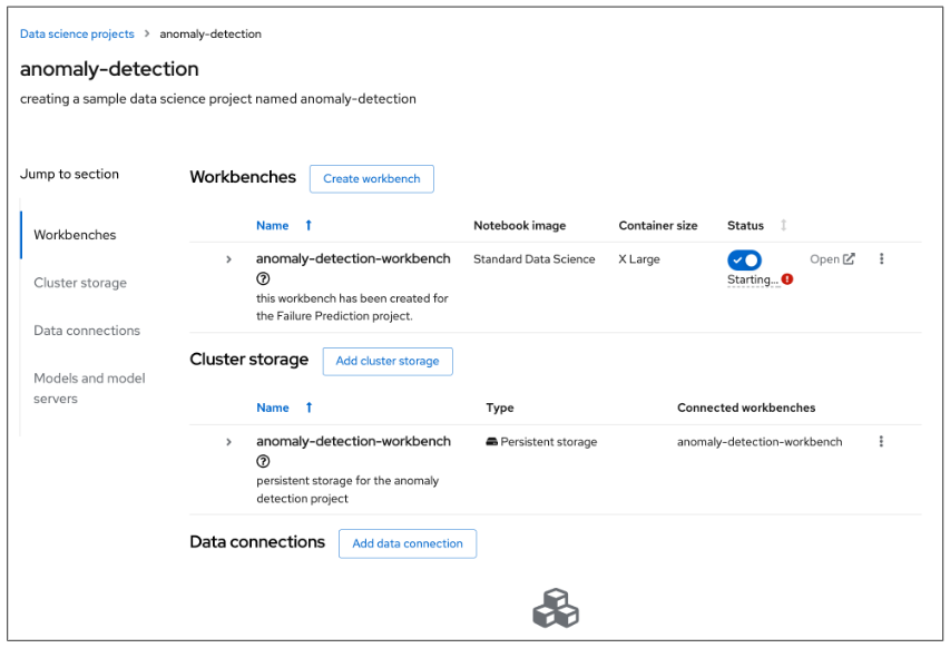
After creating the workbench, you will return to the anomaly-detection project page. (Figure 8)

Notice that a red exclamation appears under the status indicator in Figure 9. If we hover over that icon, we can see that an “insufficient memory” error has occurred.  

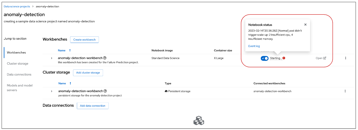
Looking closely at the error message, it appears that we don’t have enough resources; we chose a larger storage size than was available in our container. To resolve this error, we  need to edit the cluster storage so that it does not exceed our container size.

Once we have our workbench and cluster storage set up, we can add data connections. Click the Add data connection button to open the data connection configuration window. (Figure 10)

Within this window, as shown in Figure 11, you can add the following items: 

• Name
• AWS_ACCESS_KEY_ID
• AWS_SECRET_ACCESS_KEY
• AWS_S3_ENDPOINT
• AWS_DEFAULT_REGION
• AWS_S3_BUCKET

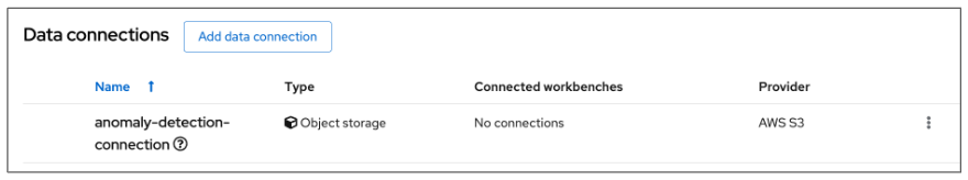
After completing the required fields, click Add data connection. You should now see the data connection displayed in the main project window. (Figure 12)

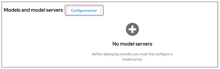
After creating the data connection, you can configure your model server. Select Configure server. (Figure 13)

In the pop-up window that appears, as in Figure 14, you can specify the following details:

• How many model server replicas to deploy
• Model server size (compute resources per replica)
• Model route
• Token authorization

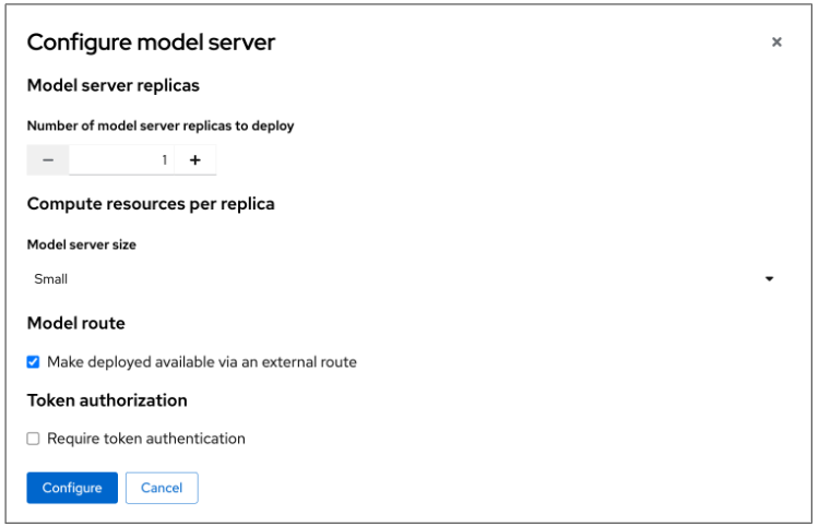
After adding and selecting options within the Configure model server pop-up window, click Configure to configure the model server.

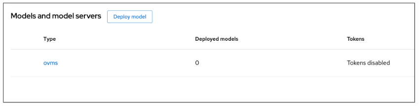
Your data science project overview shows that your model server has been configured with the default OpenVINO Model Server (ovms), as shown in Figure 15.

Once you have set up your model server, you can deploy your model. From the main Red Hat OpenShift Data Science dashboard, choose Model Serving. (Figure 16)

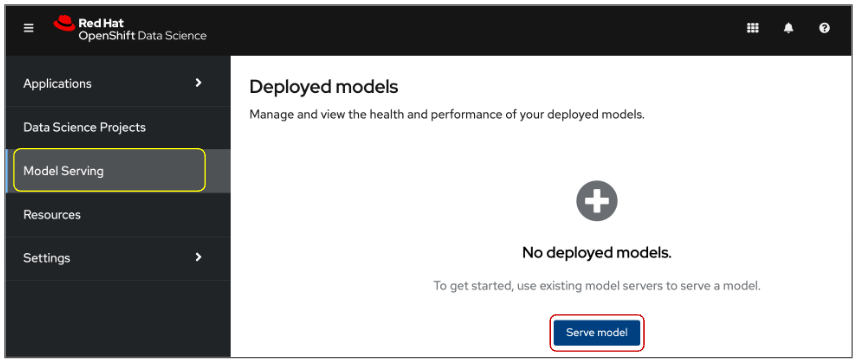
To add a model to be served, click the Serve model button. Doing so will initiate the Deploy model pop-up window. (Figure 17)

You can now use your existing data science project configurations to help you deploy your model. Notice that you can select the anomaly-detection project that we created previously. You can also choose the anomaly-detection-connection connection that you created earlier in your data science project!

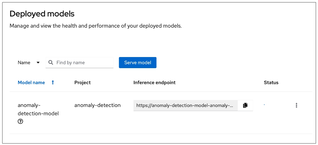
When you are ready to deploy your model, select the Deploy button. When you return to the Deployed models page, you will see your newly deployed model. (Figure 18)

This concludes our learning path on creating a data science project.