Build, train, and run your PyTorch model

To really dive into AI, you need one of the many frameworks provided for these tasks. PyTorch is an optimized tensor library primarily used for deep learning applications that combine the use of GPUs with CPUs. It is an open source machine learning library for Python, mainly developed by the Facebook AI Research team.

PyTorch is one of the most widely used machine learning libraries, others being TensorFlow and Keras. PyTorch uses dynamic computation, which allows greater flexibility in building complex architectures. We will use the torch and scikit-learn (sklearn) libraries to build and train our model.

We will be working through the following steps:

1. Reloading the data and creating a data frame.
2. Creating data sets for model training and testing.
3. Creating a PyTorch model.
4. Compiling and training the model.
5. Testing the model.
6. Saving the model.

Reload the data and create a dataframe

Open the 02-model-development.ipynb notebook. This notebook covers some of the data preparation required, as well as training and evaluating the model.

Since this is a new notebook, you need to load the diabetes data set and create a dataframe, as follows:

data_file_name = 'data/diabetes.csv'
    df  = pd.read_csv(data_file_name)

You are now ready to create data sets for training and testing.

Create data sets for model training and testing

Before you can train the model, you need to divide the data into training and testing data sets. Use sklearn's train_test_split method to split the data set into random train and test subsets:

X_train,X_test,y_train,y_test = train_test_split(X,y , test_size =0.2,random_state=0)

Once you have done this, create tensors. Tensors are specialized data structures similar to arrays and matrices but with potentially many dimensions. In PyTorch, you can use tensors to encode the inputs and outputs of a model, as well as the model's parameters. This notebook initiates the tensors directly from the data.

# Creating Tensors (multidimensional matrix) x-input data  y-output data
    X_train           = torch.FloatTensor(X_train.values)
    X_test            = torch.FloatTensor(X_test.values)
    y_train           = torch.LongTensor(y_train.values)
    y_test            = torch.LongTensor(y_test.values)

Now you are ready to create your model.

Create a PyTorch model 

To prepare for creating a Python (.py) file to house your model and code, put your model into a class called ANN_model, that you can use later in your .py file:

#Create the Model
    class ANN_model(nn.Module):
        def __init__(self,input_features=8,hidden1=20, hidden2=10,out_features=2):
            super().__init__()
            self.f_connected1 = nn.Linear(input_features,hidden1)
            self.f_connected2 = nn.Linear(hidden1,hidden2)
            self.out = nn.Linear(hidden2,out_features)
        def forward(self,x):
            x = F.relu(self.f_connected1(x))
            x = F.relu(self.f_connected2(x))
            x = self.out(x)
            return x
        def save(self, model_path):
            torch.save(model.state_dict(), model_path)
        def load(self, model_path):
            self.load_state_dict(torch.load(model_path))
            self.eval()

Compile and train the model

After creating your model, you need to compile it and determine its accuracy. In this notebook, we decided to train our model for more than one epoch. An epoch is the measure of the number of times all training data is used once to update the model parameters. We set our epoch to 500:

loss_function = nn.CrossEntropyLoss()   
    optimizer = torch.optim.Adam(model.parameters(),lr=0.01)  
    epochs=500
    final_losses=[]
    for i in range(epochs):
        i= i+1
        y_pred=model.forward(X_train)
        loss=loss_function(y_pred,y_train)
        final_losses.append(loss)
        #if i % 10 == 1:
        #    print("Epoch number: {} and the loss : {}".format(i,loss.item()))
        optimizer.zero_grad()
        loss.backward()
        optimizer.step()
    

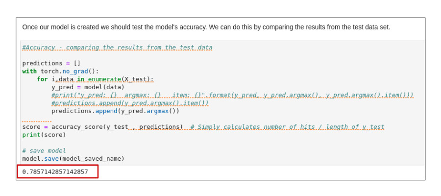
Now check the model’s accuracy by comparing its results to those from the test data (Figure 14).

One of the things you could do to improve model accuracy is to normalize the model. Let’s set this task aside for now. We’ll try out the model in its current form next.

Test the model

Now that you have a working model and feel confident about its accuracy, you are ready to test it. Testing is critical to ensure that the model will generalize to data it hasn't seen before. In this case, we want the accuracy and loss to be fairly close to the values we saw at the end of the training. If they're not, our model is probably overfitted to the training data to some extent, and won't perform well on data it hasn't seen before.

Note that no AI is perfect, and this is a departure from traditional computer science, where results tend to be either right or wrong. This tradeoff is important to understand and why AI is not suitable for every problem. However, AI is becoming more practical and is opening up solutions to a vast set of problems that were once considered nearly intractable.

Test the model using the predict() method created in the notebook:

def predict(dataset):
        predict_data = dataset
        predict_data_tensor = torch.tensor(predict_data) 
        prediction_value    = ann_model(predict_data_tensor)
        # Dict for textual display of prediction
        outcomes            = {0: 'No diabetes',1:'Diabetes Predicted'}
        # From the prediction tensor, get index of the max value ( 0 or 1)
        prediction_index   = prediction_value.argmax().item()
        prediction = outcomes[prediction_index]
        #return(outcomes[prediction_index])
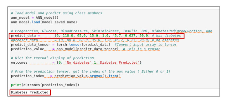
        return prediction

You can test the model with two small data sets of readings: one taken from a person with diabetes and the other from a person without diabetes. When we apply the data sets, we find that our model correctly predicts which candidate has diabetes (Figure 15).

Save the model

Finally, you need to save your model out to storage, because you'll be reusing the model in a later notebook. We will be using PyTorch.org’s recommendation for saving a PyTorch model.

Saving the model’s state_dict with the torch.save() function gives you the most flexibility for restoring the model later. It is PyTorch’s recommended method for saving models because only the trained model’s learned parameters really need to be saved. 

Note: When saving and loading a model, you can save the entire module using Python’s pickle module. This approach has the most intuitive syntax and involves the least amount of code. The disadvantage of this approach is that the serialized data is bound to the specific classes and the exact directory structure used when the model is saved. The reason for this is that pickle does not save the model class itself. Rather, it saves a path to the file containing the class, which is used during load time. Because of this, your code can break in various ways when used in other projects or after refactoring. 

PyTorch’s recommended steps for saving a model are the following:

1. Import all necessary libraries (e.g., torch) for loading the model
2. Define and initialize the neural network.
3. Initialize the optimizer.
4. Save and load the model via state_dict.
5. Save and load the entire model.

For this recipe, we will use torch and its subsidiary torch.nn.

1. Import the following libraries for loading (and saving) our PyTorch model:

import torch
    import torch.nn as nn
    import torch.nn.functional as F

2. Define and initialize the neural network:

class ANN_model(nn.Module):
        def __init__(self,input_features=8,hidden1=20, hidden2=10,out_features=2):
            super().__init__()
            self.f_connected1 = nn.Linear(input_features,hidden1)
            self.f_connected2 = nn.Linear(hidden1,hidden2)
            self.out          = nn.Linear(hidden2,out_features)
            
        def forward(self,x):
            x = F.relu(self.f_connected1(x))
            x = F.relu(self.f_connected2(x))
            x = self.out(x)
            return x
        def save(self, model_path):
            torch.save(model.state_dict(), model_path)
        def load(self, model_path):
            self.load_state_dict(torch.load(model_path))
            self.eval()

3. Initialize the optimizer. We will use Adam: 

optimizer     =
    torch.optim.Adam(model.parameters(),lr=0.01)

4. Save and load the model via state_dict:

 def save(self, model_path):
            torch.save(model.state_dict(), model_path)
     def load(self, model_path):
            self.load_state_dict(torch.load(model_path))
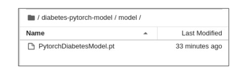
            self.eval()

A common PyTorch convention is to save models using either a .pt or .pth file extension. We have used .pt (Figure 16).

 This is the conclusion to this learning path. In the next learning path, we will continue working with this model.  We will perform normalization, further feature extraction, then deploy the model as an intelligent application.