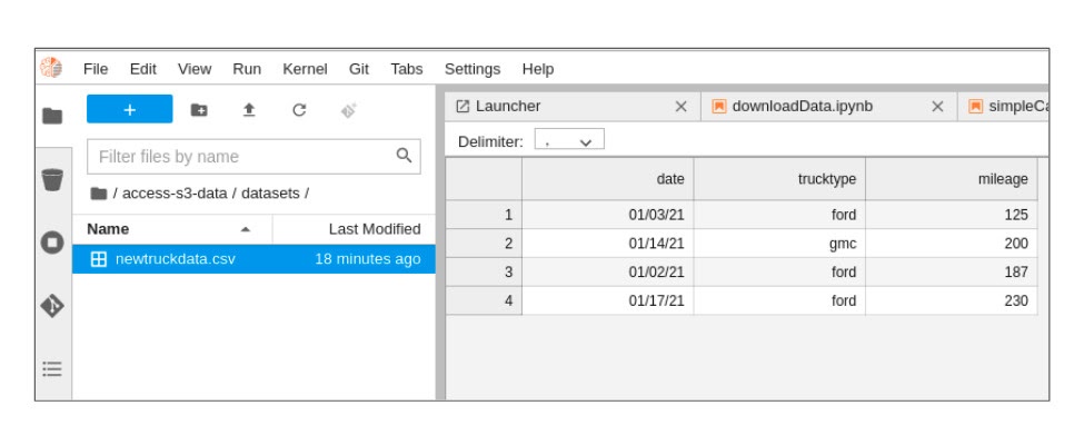
Figure 10. The user interface shows the contents of the newtruckdata.csv file.
Page

Double-click the 'newtruckdata.csv' file. File contents should appear as shown in Figure 10.
Since you now have data, you can open the next Jupyter notebook, simpleCalc.ipynb, and perform the following operations:
Double-click the simpleCalc.ipynb file. When you execute the cells in the notebook, results appear like the ones shown in Figure 11.
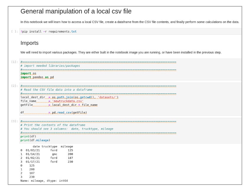
The cells in Figure 11 show the mileage of four vehicles. In the next cell, we calculate total mileage, total rows (number of vehicles) and the average mileage for all vehicles. Execute the “Perform Calculations” cell to see basic calculations performed on the data (Figure 12).
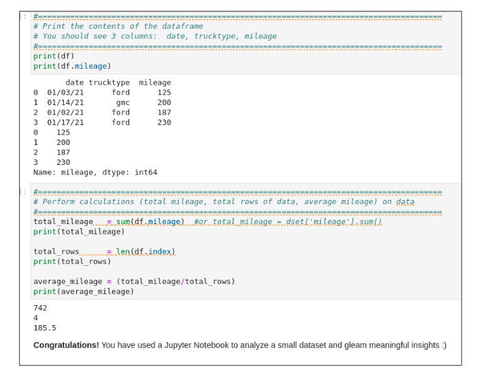
Success! You have analyzed your run results using Red Hat OpenShift Data Science.

Build here. Go anywhere.
We serve the builders. The problem solvers who create careers with code.
Join us if you’re a developer, software engineer, web designer, front-end designer, UX designer, computer scientist, architect, tester, product manager, project manager or team lead.