Page
How to examine GPU resources with PyTorch

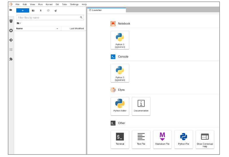
Welcome to JupyterLab!
After starting your server, three sections appear in JupyterLab's launcher:
- Notebook
- Console
- Other
On the left side of the navigation pane, locate the Name explorer panel (Figure 3). This panel is where you can create and manage your project directories.
Clone a GitHub Repository
Now it's time to populate your JupyterLab notebook with a GitHub repository. Select the Git/Clone a Repository menu option. A dialog box will appear (Figure 4).

Enter the URL of the repository for this learning path, which is https://github.com/rh-aiservices-bu/getting-started-with-gpus, and select Clone to clone the getting-started-with-gpus repository.
Note: GitHub may ask for your credentials. Follow the GitHub authentication process, then select Ok.
The getting-started-with-gpus repository contents
After you've cloned your repository, the getting-started-with-gpus repository contents appear in a directory under the Name pane (Figure 5). The directory contains several notebooks as .ipnyb files, along with a standard license and README file.
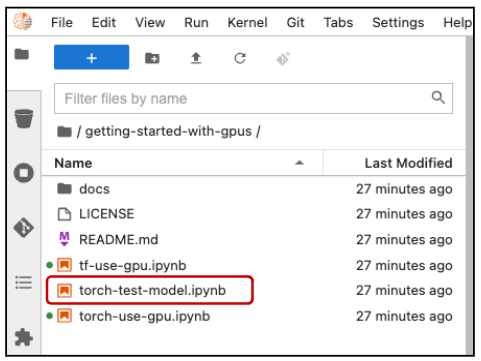
Double-click the torch-use-gpu.ipynb file to open this notebook. The screen shown by the notebook looks like Figure 6.

This notebook handles the following tasks:
- Importing torch libraries (utilities).
- Listing available GPUs.
- Checking that GPUs are enabled.
- Assigning a GPU device and retrieve the GPU name.
- Loading vectors, matrices, and data onto a GPU.
- Loading a neural network model onto a GPU.
- Training the neural network model.
Start by importing the various torch and torchvision utilities:
import torch
import torch.nn as nn
import torch.nn.functional as F
from torch.utils.data import TensorDataset
import torch.optim as optim
import torchvision
from torchvision import datasets
import torchvision.transforms as transforms
import matplotlib.pyplot as plt
from tqdm import tqdm
Once the utilities are loaded, determine how many GPUs are available:
torch.cuda.is_available() # Do we have a GPU? Should return True.
torch.cuda.device_count() # How many GPUs do we have access to?
If you see ‘0’ GPU(s) available, go back to the Notebook server options and check that you selected at least one GPU. You can change options by selecting File→Hub Control Panel from the drop-down menus (Figure 7).
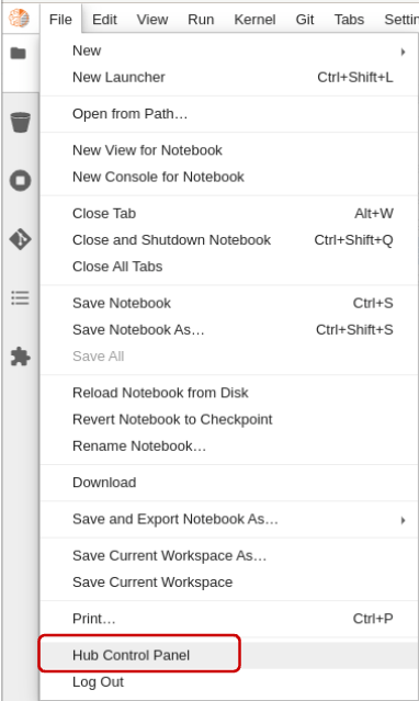
Once in the Hub Control Panel, you can check whether you selected any GPUs. If you choose a GPU, but it is not enabled in your notebook, contact the personnel that set up your GPU cluster.
When you have confirmed that a GPU device is available for use, assign a GPU device and retrieve the GPU name:
device = torch.device("cuda:0" if torch.cuda.is_available() else "cpu")
print(device)  # Check which device we got
torch.cuda.get_device_name(0)
Once you have assigned the first GPU device to your device variable, you are ready to work with the GPU. Let’s start working with the GPU by loading vectors, matrices, and data:
X_train = torch.IntTensor([0, 30, 50, 75, 70])  # Initialize a Tensor of Integers with no device specified
print(X_train.is_cuda, ",", X_train.device)  # Check which device Tensor is created on
# Move the Tensor to the device we want to use
X_train = X_train.cuda()
# Alternative method: specify the device using the variable
# X_train = X_train.to(device)
# Confirm that the Tensor is on the GPU now
print(X_train.is_cuda, ",", X_train.device)
# Alternative method: Initialize the Tensor directly on a specific device.
X_test = torch.cuda.IntTensor([30, 40, 50], device=device)
print(X_test.is_cuda, ",", X_test.device)
After you have loaded vectors, matrices, and data onto a GPU, load a neural network model:
# Here is a basic fully connected neural network built in Torch.
# If we want to load it / train it on our GPU, we must first put it on the GPU
# Otherwise it will remain on CPU by default.

batch_size = 100

class SimpleNet(nn.Module):
    def __init__(self):
        super(SimpleNet, self).__init__()
        self.fc1 = nn.Linear(784, 784)
        self.fc2 = nn.Linear(784, 10)

    def forward(self, x):
        x = x.view(batch_size, -1)
        x = self.fc1(x)
        x = F.relu(x)
        x = self.fc2(x)
        output = F.softmax(x, dim=1)
        return output
model = SimpleNet().to(device) # Load the neural network model onto the GPU
After the model has been loaded onto the GPU, train it on a data set. For this example, we will use the FashionMNIST data set:
"""
    Data loading, train and test set via the PyTorch dataloader.
"""
# Transform our data into Tensors to normalize the data
train_transform=transforms.Compose([
        transforms.ToTensor(),
        transforms.Normalize((0.1307,), (0.3081,))
        ])

test_transform=transforms.Compose([
        transforms.ToTensor(),
        transforms.Normalize((0.1307,), (0.3081,)),
        ])

# Set up a training data set
trainset = datasets.FashionMNIST('./data', train=True, download=True,
                  transform=train_transform)
train_loader = torch.utils.data.DataLoader(trainset, batch_size=batch_size,
                                          shuffle=False, num_workers=2)

# Set up a test data set
testset = datasets.FashionMNIST('./data', train=False,
                  transform=test_transform)
test_loader = torch.utils.data.DataLoader(testset, batch_size=batch_size,
                                        shuffle=False, num_workers=2)
Once the FashionMNIST data set has been downloaded, you can take a look at the dictionary and sample its content. A few of the data set’s pictures are shown in Figure 8.
# A dictionary to map our class numbers to their items.
labels_map = {
    0: "T-Shirt",
    1: "Trouser",
    2: "Pullover",
    3: "Dress",
    4: "Coat",
    5: "Sandal",
    6: "Shirt",
    7: "Sneaker",
    8: "Bag",
    9: "Ankle Boot",
}

# Plotting 9 random different items from the training data set, trainset.
figure = plt.figure(figsize=(8, 8))
for i in range(1, 3 * 3 + 1):
    sample_idx = torch.randint(len(trainset), size=(1,)).item()
    img, label = trainset[sample_idx]
    figure.add_subplot(3, 3, i)
    plt.title(labels_map[label])
    plt.axis("off")
    plt.imshow(img.view(28,28), cmap="gray")
plt.show()
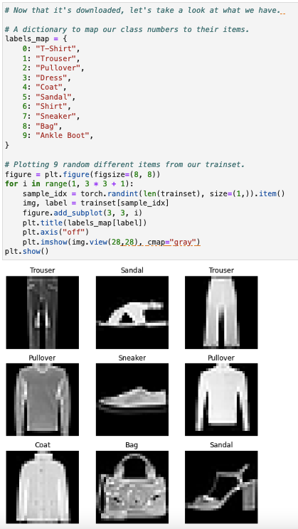
There are ten classes of fashion items (e.g. shirt, shoes, and so on). Our goal is to identify which class each picture falls into. Now you can train the model and determine how well it classifies the items:
def train(model, device, train_loader, optimizer, epoch):
    """Model training function"""
    model.train()
    print(device)
    for batch_idx, (data, target) in tqdm(enumerate(train_loader)):
        data, target = data.to(device), target.to(device)
        optimizer.zero_grad()
        output = model(data)
        loss = F.nll_loss(output, target)
        loss.backward()
        optimizer.step()
def test(model, device, test_loader):
    """Model evaluating function"""
    model.eval()
    test_loss = 0
    correct = 0
    with torch.no_grad():
        for data, target in test_loader:
            data, target = data.to(device), target.to(device)
            output = model(data)
            test_loss += F.nll_loss(output, target, reduction='sum').item()  # sum up batch loss
            pred = output.argmax(dim=1, keepdim=True)  # get the index of the max log-probability
            correct += pred.eq(target.view_as(pred)).sum().item()

    test_loss /= len(test_loader.dataset)

    print('\nTest set: Average loss: {:.4f}, Accuracy: {}/{} ({:.0f}%)\n'.format(
        test_loss, correct, len(test_loader.dataset),
        100. * correct / len(test_loader.dataset)))
def test(model, device, test_loader):
    model.eval()
    test_loss = 0
    correct = 0
    # Use the no_grad method to increase computation speed
    # since computing the gradient is not necessary in this step.
    with torch.no_grad():
        for data, target in test_loader:
            data, target = data.to(device), target.to(device)
            output = model(data)
            test_loss += F.nll_loss(output, target, reduction='sum').item()  # sum up batch loss
            pred = output.argmax(dim=1, keepdim=True)  # get the index of the max log-probability
            correct += pred.eq(target.view_as(pred)).sum().item()

    test_loss /= len(test_loader.dataset)

    print('\nTest set: Average loss: {:.4f}, Accuracy: {}/{} ({:.0f}%)\n'.format(
        test_loss, correct, len(test_loader.dataset),
        100. * correct / len(test_loader.dataset)))
# number of  training 'epochs'
EPOCHS = 5
# our optimization strategy used in training.
optimizer = optim.Adadelta(model.parameters(), lr=0.01)
for epoch in range(1, EPOCHS + 1):
        print( f"EPOCH: {epoch}")
        train(model, device, train_loader, optimizer, epoch)
        test(model, device, test_loader)
As the model is trained, you can follow along as its accuracy increases from 63 to 72 percent. (Your accuracies might differ, because accuracy can depend on the random initialization of weights.)
for epoch in range(1, EPOCHS + 1):
        print( f"EPOCH: {epoch}")
        train(model, device, train_loader, optimizer, epoch)
        test(model, device, test_loader)
Once the model is trained, save it locally:
# Saving the model's weights!
torch.save(model.state_dict(), "mnist_fashion_SimpleNet.pt")
Proceed to the next section, “Load and run a PyTorch model.”
